Compare commits
8 Commits
main
...
distribute
| Author | SHA1 | Date | |
|---|---|---|---|
|
|
d6a375ea34 | ||
|
|
a91577319e | ||
|
|
5ff45521c5 | ||
|
|
d62bbff1f0 | ||
|
|
7091378d35 | ||
|
|
70aacb3d75 | ||
|
|
b9f761d256 | ||
|
|
aca1e0698b |
73
.github/workflows/sync-from-gitea-deploy.yml
vendored
Normal file
73
.github/workflows/sync-from-gitea-deploy.yml
vendored
Normal file
@@ -0,0 +1,73 @@
|
|||||||
|
name: Sync from Gitea (distribute→distribute, keep workflow)
|
||||||
|
|
||||||
|
on:
|
||||||
|
schedule:
|
||||||
|
# 2 times per day (UTC): 7:00, 11:00
|
||||||
|
- cron: '0 7,11 * * *'
|
||||||
|
workflow_dispatch: {}
|
||||||
|
|
||||||
|
permissions:
|
||||||
|
contents: write # allow pushing with GITHUB_TOKEN
|
||||||
|
|
||||||
|
jobs:
|
||||||
|
mirror:
|
||||||
|
runs-on: ubuntu-latest
|
||||||
|
|
||||||
|
steps:
|
||||||
|
- name: Check out GitHub repo
|
||||||
|
uses: actions/checkout@v4
|
||||||
|
with:
|
||||||
|
fetch-depth: 0
|
||||||
|
|
||||||
|
- name: Fetch from Gitea
|
||||||
|
env:
|
||||||
|
GITEA_URL: ${{ secrets.GITEA_URL }}
|
||||||
|
GITEA_USER: ${{ secrets.GITEA_USERNAME }}
|
||||||
|
GITEA_TOKEN: ${{ secrets.GITEA_TOKEN }}
|
||||||
|
run: |
|
||||||
|
# Build authenticated Gitea URL: https://USER:TOKEN@...
|
||||||
|
AUTH_URL="${GITEA_URL/https:\/\//https:\/\/$GITEA_USER:$GITEA_TOKEN@}"
|
||||||
|
|
||||||
|
git remote add gitea "$AUTH_URL"
|
||||||
|
git fetch gitea --prune
|
||||||
|
|
||||||
|
- name: Update distribute from gitea/distribute, keep workflow, and force-push
|
||||||
|
env:
|
||||||
|
GH_TOKEN: ${{ secrets.GITHUB_TOKEN }}
|
||||||
|
GH_REPO: ${{ github.repository }}
|
||||||
|
run: |
|
||||||
|
# Configure identity for commits made by this workflow
|
||||||
|
git config user.name "github-actions[bot]"
|
||||||
|
git config user.email "github-actions[bot]@users.noreply.github.com"
|
||||||
|
|
||||||
|
# Authenticated push URL for GitHub
|
||||||
|
git remote set-url origin "https://x-access-token:${GH_TOKEN}@github.com/${GH_REPO}.git"
|
||||||
|
|
||||||
|
WF_PATH=".github/workflows/sync-from-gitea.yml"
|
||||||
|
|
||||||
|
# If the workflow exists in the current checkout, save a copy
|
||||||
|
if [ -f "$WF_PATH" ]; then
|
||||||
|
mkdir -p /tmp/gh-workflows
|
||||||
|
cp "$WF_PATH" /tmp/gh-workflows/
|
||||||
|
fi
|
||||||
|
|
||||||
|
# Reset local 'distribute' to exactly match gitea/distribute
|
||||||
|
if git show-ref --verify --quiet refs/remotes/gitea/distribute; then
|
||||||
|
git checkout -B distribute gitea/distribute
|
||||||
|
else
|
||||||
|
echo "No gitea/distribute found, nothing to sync."
|
||||||
|
exit 0
|
||||||
|
fi
|
||||||
|
|
||||||
|
# Restore the workflow into the new HEAD and commit if needed
|
||||||
|
if [ -f "/tmp/gh-workflows/sync-from-gitea.yml" ]; then
|
||||||
|
mkdir -p .github/workflows
|
||||||
|
cp /tmp/gh-workflows/sync-from-gitea.yml "$WF_PATH"
|
||||||
|
git add "$WF_PATH"
|
||||||
|
if ! git diff --cached --quiet; then
|
||||||
|
git commit -m "Inject GitHub sync workflow"
|
||||||
|
fi
|
||||||
|
fi
|
||||||
|
|
||||||
|
# Force-push distribute so GitHub mirrors Gitea + workflow
|
||||||
|
git push origin distribute --force
|
||||||
2
.github/workflows/sync-from-gitea.yml
vendored
2
.github/workflows/sync-from-gitea.yml
vendored
@@ -3,7 +3,7 @@ name: Sync from Gitea (main→main, keep workflow)
|
|||||||
on:
|
on:
|
||||||
schedule:
|
schedule:
|
||||||
# 2 times per day (UTC): 7:00, 11:00
|
# 2 times per day (UTC): 7:00, 11:00
|
||||||
- cron: '0 19,23 * * *'
|
- cron: '0 7,11 * * *'
|
||||||
workflow_dispatch: {}
|
workflow_dispatch: {}
|
||||||
|
|
||||||
permissions:
|
permissions:
|
||||||
|
|||||||
301
.gitignore
vendored
301
.gitignore
vendored
@@ -1,152 +1,149 @@
|
|||||||
# Logs
|
# Logs
|
||||||
logs
|
logs
|
||||||
*.log
|
*.log
|
||||||
npm-debug.log*
|
npm-debug.log*
|
||||||
yarn-debug.log*
|
yarn-debug.log*
|
||||||
yarn-error.log*
|
yarn-error.log*
|
||||||
lerna-debug.log*
|
lerna-debug.log*
|
||||||
.pnpm-debug.log*
|
.pnpm-debug.log*
|
||||||
|
|
||||||
# Diagnostic reports (https://nodejs.org/api/report.html)
|
# Diagnostic reports (https://nodejs.org/api/report.html)
|
||||||
report.[0-9]*.[0-9]*.[0-9]*.[0-9]*.json
|
report.[0-9]*.[0-9]*.[0-9]*.[0-9]*.json
|
||||||
|
|
||||||
# Runtime data
|
# Runtime data
|
||||||
pids
|
pids
|
||||||
*.pid
|
*.pid
|
||||||
*.seed
|
*.seed
|
||||||
*.pid.lock
|
*.pid.lock
|
||||||
|
|
||||||
# Directory for instrumented libs generated by jscoverage/JSCover
|
# Directory for instrumented libs generated by jscoverage/JSCover
|
||||||
lib-cov
|
lib-cov
|
||||||
|
|
||||||
# Coverage directory used by tools like istanbul
|
# Coverage directory used by tools like istanbul
|
||||||
coverage
|
coverage
|
||||||
*.lcov
|
*.lcov
|
||||||
|
|
||||||
# nyc test coverage
|
# nyc test coverage
|
||||||
.nyc_output
|
.nyc_output
|
||||||
|
|
||||||
# Grunt intermediate storage (https://gruntjs.com/creating-plugins#storing-task-files)
|
# Grunt intermediate storage (https://gruntjs.com/creating-plugins#storing-task-files)
|
||||||
.grunt
|
.grunt
|
||||||
|
|
||||||
# Bower dependency directory (https://bower.io/)
|
# Bower dependency directory (https://bower.io/)
|
||||||
bower_components
|
bower_components
|
||||||
|
|
||||||
# node-waf configuration
|
# node-waf configuration
|
||||||
.lock-wscript
|
.lock-wscript
|
||||||
|
|
||||||
# Compiled binary addons (https://nodejs.org/api/addons.html)
|
# Compiled binary addons (https://nodejs.org/api/addons.html)
|
||||||
build/Release
|
build/Release
|
||||||
|
|
||||||
# Dependency directories
|
# Dependency directories
|
||||||
node_modules/
|
node_modules/
|
||||||
jspm_packages/
|
jspm_packages/
|
||||||
|
|
||||||
# Snowpack dependency directory (https://snowpack.dev/)
|
# Snowpack dependency directory (https://snowpack.dev/)
|
||||||
web_modules/
|
web_modules/
|
||||||
|
|
||||||
# TypeScript cache
|
# TypeScript cache
|
||||||
*.tsbuildinfo
|
*.tsbuildinfo
|
||||||
|
|
||||||
# Optional npm cache directory
|
# Optional npm cache directory
|
||||||
.npm
|
.npm
|
||||||
|
|
||||||
# Optional eslint cache
|
# Optional eslint cache
|
||||||
.eslintcache
|
.eslintcache
|
||||||
|
|
||||||
# Optional stylelint cache
|
# Optional stylelint cache
|
||||||
.stylelintcache
|
.stylelintcache
|
||||||
|
|
||||||
# Microbundle cache
|
# Microbundle cache
|
||||||
.rpt2_cache/
|
.rpt2_cache/
|
||||||
.rts2_cache_cjs/
|
.rts2_cache_cjs/
|
||||||
.rts2_cache_es/
|
.rts2_cache_es/
|
||||||
.rts2_cache_umd/
|
.rts2_cache_umd/
|
||||||
|
|
||||||
# Optional REPL history
|
# Optional REPL history
|
||||||
.node_repl_history
|
.node_repl_history
|
||||||
|
|
||||||
# Output of 'npm pack'
|
# Output of 'npm pack'
|
||||||
*.tgz
|
*.tgz
|
||||||
|
|
||||||
# Yarn Integrity file
|
# Yarn Integrity file
|
||||||
.yarn-integrity
|
.yarn-integrity
|
||||||
|
|
||||||
# dotenv environment variable files
|
# dotenv environment variable files
|
||||||
.env
|
.env
|
||||||
.env.development.local
|
.env.development.local
|
||||||
.env.test.local
|
.env.test.local
|
||||||
.env.production.local
|
.env.production.local
|
||||||
.env.local
|
.env.local
|
||||||
|
|
||||||
# parcel-bundler cache (https://parceljs.org/)
|
# parcel-bundler cache (https://parceljs.org/)
|
||||||
.cache
|
.cache
|
||||||
.parcel-cache
|
.parcel-cache
|
||||||
|
|
||||||
# Next.js build output
|
# Next.js build output
|
||||||
.next
|
.next
|
||||||
out
|
out
|
||||||
|
|
||||||
# Nuxt.js build / generate output
|
# Nuxt.js build / generate output
|
||||||
.nuxt
|
.nuxt
|
||||||
dist
|
dist
|
||||||
|
|
||||||
# Gatsby files
|
# Gatsby files
|
||||||
.cache/
|
.cache/
|
||||||
# Comment in the public line in if your project uses Gatsby and not Next.js
|
# Comment in the public line in if your project uses Gatsby and not Next.js
|
||||||
# https://nextjs.org/blog/next-9-1#public-directory-support
|
# https://nextjs.org/blog/next-9-1#public-directory-support
|
||||||
# public
|
# public
|
||||||
|
|
||||||
# vuepress build output
|
# vuepress build output
|
||||||
.vuepress/dist
|
.vuepress/dist
|
||||||
|
|
||||||
# vuepress v2.x temp and cache directory
|
# vuepress v2.x temp and cache directory
|
||||||
.temp
|
.temp
|
||||||
.cache
|
.cache
|
||||||
|
|
||||||
# Docusaurus cache and generated files
|
# Docusaurus cache and generated files
|
||||||
.docusaurus
|
.docusaurus
|
||||||
|
|
||||||
# Serverless directories
|
# Serverless directories
|
||||||
.serverless/
|
.serverless/
|
||||||
|
|
||||||
# FuseBox cache
|
# FuseBox cache
|
||||||
.fusebox/
|
.fusebox/
|
||||||
|
|
||||||
# DynamoDB Local files
|
# DynamoDB Local files
|
||||||
.dynamodb/
|
.dynamodb/
|
||||||
|
|
||||||
# TernJS port file
|
# TernJS port file
|
||||||
.tern-port
|
.tern-port
|
||||||
|
|
||||||
# Stores VSCode versions used for testing VSCode extensions
|
# Stores VSCode versions used for testing VSCode extensions
|
||||||
.vscode-test
|
.vscode-test
|
||||||
|
|
||||||
# yarn v2
|
# yarn v2
|
||||||
.yarn/cache
|
.yarn/cache
|
||||||
.yarn/unplugged
|
.yarn/unplugged
|
||||||
.yarn/build-state.yml
|
.yarn/build-state.yml
|
||||||
.yarn/install-state.gz
|
.yarn/install-state.gz
|
||||||
.pnp.*
|
.pnp.*
|
||||||
|
|
||||||
# vscode
|
# vscode
|
||||||
.vscode
|
.vscode
|
||||||
|
|
||||||
# analytics
|
# analytics
|
||||||
analyze/
|
analyze/
|
||||||
|
|
||||||
# heapsnapshot
|
# heapsnapshot
|
||||||
*.heapsnapshot
|
*.heapsnapshot
|
||||||
|
|
||||||
# turbo
|
# turbo
|
||||||
.turbo/
|
.turbo/
|
||||||
|
|
||||||
# pagefind postbuild
|
# pagefind postbuild
|
||||||
public/_pagefind/
|
public/_pagefind/
|
||||||
public/sitemap.xml
|
public/sitemap.xml
|
||||||
|
|
||||||
# npm package lock file for different platforms
|
# npm package lock file for different platforms
|
||||||
package-lock.json
|
package-lock.json
|
||||||
|
|
||||||
# generated
|
|
||||||
mcp-worker/generated
|
|
||||||
79
README.md
79
README.md
@@ -1,53 +1,38 @@
|
|||||||
# NoteNextra
|
# NoteNextra
|
||||||
|
|
||||||
Static note sharing site with minimum care
|
Static note sharing site with minimum care
|
||||||
|
|
||||||
This site is powered by
|
This site is powered by
|
||||||
|
|
||||||
- [Next.js](https://nextjs.org/)
|
- [Next.js](https://nextjs.org/)
|
||||||
- [Nextra](https://nextra.site/)
|
- [Nextra](https://nextra.site/)
|
||||||
- [Tailwind CSS](https://tailwindcss.com/)
|
- [Tailwind CSS](https://tailwindcss.com/)
|
||||||
- [Vercel](https://vercel.com/)
|
- [Vercel](https://vercel.com/)
|
||||||
|
|
||||||
## Deployment
|
## Deployment
|
||||||
|
|
||||||
### Deploying to Vercel
|
### Deploying to Vercel
|
||||||
|
|
||||||
[](https://vercel.com/new/clone?repository-url=https%3A%2F%2Fgithub.com%2FTrance-0%2FNotechondria)
|
[](https://vercel.com/new/clone?repository-url=https%3A%2F%2Fgithub.com%2FTrance-0%2FNotechondria)
|
||||||
|
|
||||||
_Warning: This project is not suitable for free Vercel plan. There is insufficient memory for the build process._
|
_Warning: This project is not suitable for free Vercel plan. There is insufficient memory for the build process._
|
||||||
|
|
||||||
### Deploying to Cloudflare Pages
|
### Deploying to Cloudflare Pages
|
||||||
|
|
||||||
[](https://deploy.workers.cloudflare.com/?url=https://github.com/Trance-0/Notechondria)
|
[](https://deploy.workers.cloudflare.com/?url=https://github.com/Trance-0/Notechondria)
|
||||||
|
|
||||||
### Deploying as separated docker services
|
### Deploying as separated docker services
|
||||||
|
|
||||||
Considering the memory usage for this project, it is better to deploy it as separated docker services.
|
Considering the memory usage for this project, it is better to deploy it as separated docker services.
|
||||||
|
|
||||||
```bash
|
```bash
|
||||||
docker-compose up -d -f docker/docker-compose.yaml
|
docker-compose up -d -f docker/docker-compose.yaml
|
||||||
```
|
```
|
||||||
|
|
||||||
### Snippets
|
### Snippets
|
||||||
|
|
||||||
Update dependencies
|
Update dependencies
|
||||||
|
|
||||||
```bash
|
```bash
|
||||||
npx npm-check-updates -u
|
npx npm-check-updates -u
|
||||||
```
|
```
|
||||||
|
|
||||||
### MCP access to notes
|
|
||||||
|
|
||||||
This repository includes a minimal MCP server that exposes the existing `content/` notes as a knowledge base for AI tools over stdio.
|
|
||||||
|
|
||||||
```bash
|
|
||||||
npm install
|
|
||||||
npm run mcp:notes
|
|
||||||
```
|
|
||||||
|
|
||||||
The server exposes:
|
|
||||||
|
|
||||||
- `list_notes`
|
|
||||||
- `read_note`
|
|
||||||
- `search_notes`
|
|
||||||
@@ -1,23 +1,61 @@
|
|||||||
export default {
|
export default {
|
||||||
index: "Course Description",
|
menu: {
|
||||||
"---":{
|
title: 'Home',
|
||||||
type: 'separator'
|
type: 'menu',
|
||||||
|
items: {
|
||||||
|
index: {
|
||||||
|
title: 'Home',
|
||||||
|
href: '/'
|
||||||
|
},
|
||||||
|
about: {
|
||||||
|
title: 'About',
|
||||||
|
href: '/about'
|
||||||
|
},
|
||||||
|
contact: {
|
||||||
|
title: 'Contact Me',
|
||||||
|
href: '/contact'
|
||||||
|
}
|
||||||
|
},
|
||||||
},
|
},
|
||||||
CSE332S_L1: "Object-Oriented Programming Lab (Lecture 1)",
|
Math3200'CSE332S_link\s*:\s*(\{\s+.+\s+.+)\s+.+\s+.+\s+.+\s+(\},)'
|
||||||
CSE332S_L2: "Object-Oriented Programming Lab (Lecture 2)",
|
Math429'CSE332S_link\s*:\s*(\{\s+.+\s+.+)\s+.+\s+.+\s+.+\s+(\},)'
|
||||||
CSE332S_L3: "Object-Oriented Programming Lab (Lecture 3)",
|
Math4111'CSE332S_link\s*:\s*(\{\s+.+\s+.+)\s+.+\s+.+\s+.+\s+(\},)'
|
||||||
CSE332S_L4: "Object-Oriented Programming Lab (Lecture 4)",
|
Math4121'CSE332S_link\s*:\s*(\{\s+.+\s+.+)\s+.+\s+.+\s+.+\s+(\},)'
|
||||||
CSE332S_L5: "Object-Oriented Programming Lab (Lecture 5)",
|
Math4201'CSE332S_link\s*:\s*(\{\s+.+\s+.+)\s+.+\s+.+\s+.+\s+(\},)'
|
||||||
CSE332S_L6: "Object-Oriented Programming Lab (Lecture 6)",
|
Math416'CSE332S_link\s*:\s*(\{\s+.+\s+.+)\s+.+\s+.+\s+.+\s+(\},)'
|
||||||
CSE332S_L7: "Object-Oriented Programming Lab (Lecture 7)",
|
Math401'CSE332S_link\s*:\s*(\{\s+.+\s+.+)\s+.+\s+.+\s+.+\s+(\},)'
|
||||||
CSE332S_L8: "Object-Oriented Programming Lab (Lecture 8)",
|
CSE332S'CSE332S_link\s*:\s*(\{\s+.+\s+.+)\s+.+\s+.+\s+.+\s+(\},)'
|
||||||
CSE332S_L9: "Object-Oriented Programming Lab (Lecture 9)",
|
CSE347'CSE332S_link\s*:\s*(\{\s+.+\s+.+)\s+.+\s+.+\s+.+\s+(\},)'
|
||||||
CSE332S_L10: "Object-Oriented Programming Lab (Lecture 10)",
|
CSE442T'CSE332S_link\s*:\s*(\{\s+.+\s+.+)\s+.+\s+.+\s+.+\s+(\},)'
|
||||||
CSE332S_L11: "Object-Oriented Programming Lab (Lecture 11)",
|
CSE5313'CSE332S_link\s*:\s*(\{\s+.+\s+.+)\s+.+\s+.+\s+.+\s+(\},)'
|
||||||
CSE332S_L12: "Object-Oriented Programming Lab (Lecture 12)",
|
CSE510'CSE332S_link\s*:\s*(\{\s+.+\s+.+)\s+.+\s+.+\s+.+\s+(\},)'
|
||||||
CSE332S_L13: "Object-Oriented Programming Lab (Lecture 13)",
|
CSE559A'CSE332S_link\s*:\s*(\{\s+.+\s+.+)\s+.+\s+.+\s+.+\s+(\},)'
|
||||||
CSE332S_L14: "Object-Oriented Programming Lab (Lecture 14)",
|
CSE5519'CSE332S_link\s*:\s*(\{\s+.+\s+.+)\s+.+\s+.+\s+.+\s+(\},)'
|
||||||
CSE332S_L15: "Object-Oriented Programming Lab (Lecture 15)",
|
Swap: {
|
||||||
CSE332S_L16: "Object-Oriented Programming Lab (Lecture 16)",
|
display: 'hidden',
|
||||||
CSE332S_L17: "Object-Oriented Programming Lab (Lecture 17)"
|
theme:{
|
||||||
}
|
timestamp: true,
|
||||||
|
}
|
||||||
|
},
|
||||||
|
index: {
|
||||||
|
display: 'hidden',
|
||||||
|
theme:{
|
||||||
|
sidebar: false,
|
||||||
|
timestamp: true,
|
||||||
|
}
|
||||||
|
},
|
||||||
|
about: {
|
||||||
|
display: 'hidden',
|
||||||
|
theme:{
|
||||||
|
sidebar: false,
|
||||||
|
timestamp: true,
|
||||||
|
}
|
||||||
|
},
|
||||||
|
contact: {
|
||||||
|
display: 'hidden',
|
||||||
|
theme:{
|
||||||
|
sidebar: false,
|
||||||
|
timestamp: true,
|
||||||
|
}
|
||||||
|
}
|
||||||
|
}
|
||||||
@@ -1,18 +1,61 @@
|
|||||||
export default {
|
export default {
|
||||||
index: "Course Description",
|
menu: {
|
||||||
"---":{
|
title: 'Home',
|
||||||
type: 'separator'
|
type: 'menu',
|
||||||
|
items: {
|
||||||
|
index: {
|
||||||
|
title: 'Home',
|
||||||
|
href: '/'
|
||||||
|
},
|
||||||
|
about: {
|
||||||
|
title: 'About',
|
||||||
|
href: '/about'
|
||||||
|
},
|
||||||
|
contact: {
|
||||||
|
title: 'Contact Me',
|
||||||
|
href: '/contact'
|
||||||
|
}
|
||||||
|
},
|
||||||
},
|
},
|
||||||
Exam_reviews: "Exam reviews",
|
Math3200'CSE347_link\s*:\s*(\{\s+.+\s+.+)\s+.+\s+.+\s+.+\s+(\},)'
|
||||||
CSE347_L1: "Analysis of Algorithms (Lecture 1)",
|
Math429'CSE347_link\s*:\s*(\{\s+.+\s+.+)\s+.+\s+.+\s+.+\s+(\},)'
|
||||||
CSE347_L2: "Analysis of Algorithms (Lecture 2)",
|
Math4111'CSE347_link\s*:\s*(\{\s+.+\s+.+)\s+.+\s+.+\s+.+\s+(\},)'
|
||||||
CSE347_L3: "Analysis of Algorithms (Lecture 3)",
|
Math4121'CSE347_link\s*:\s*(\{\s+.+\s+.+)\s+.+\s+.+\s+.+\s+(\},)'
|
||||||
CSE347_L4: "Analysis of Algorithms (Lecture 4)",
|
Math4201'CSE347_link\s*:\s*(\{\s+.+\s+.+)\s+.+\s+.+\s+.+\s+(\},)'
|
||||||
CSE347_L5: "Analysis of Algorithms (Lecture 5)",
|
Math416'CSE347_link\s*:\s*(\{\s+.+\s+.+)\s+.+\s+.+\s+.+\s+(\},)'
|
||||||
CSE347_L6: "Analysis of Algorithms (Lecture 6)",
|
Math401'CSE347_link\s*:\s*(\{\s+.+\s+.+)\s+.+\s+.+\s+.+\s+(\},)'
|
||||||
CSE347_L7: "Analysis of Algorithms (Lecture 7)",
|
CSE332S'CSE347_link\s*:\s*(\{\s+.+\s+.+)\s+.+\s+.+\s+.+\s+(\},)'
|
||||||
CSE347_L8: "Analysis of Algorithms (Lecture 8)",
|
CSE347'CSE347_link\s*:\s*(\{\s+.+\s+.+)\s+.+\s+.+\s+.+\s+(\},)'
|
||||||
CSE347_L9: "Analysis of Algorithms (Lecture 9)",
|
CSE442T'CSE347_link\s*:\s*(\{\s+.+\s+.+)\s+.+\s+.+\s+.+\s+(\},)'
|
||||||
CSE347_L10: "Analysis of Algorithms (Lecture 10)",
|
CSE5313'CSE347_link\s*:\s*(\{\s+.+\s+.+)\s+.+\s+.+\s+.+\s+(\},)'
|
||||||
CSE347_L11: "Analysis of Algorithms (Lecture 11)"
|
CSE510'CSE347_link\s*:\s*(\{\s+.+\s+.+)\s+.+\s+.+\s+.+\s+(\},)'
|
||||||
}
|
CSE559A'CSE347_link\s*:\s*(\{\s+.+\s+.+)\s+.+\s+.+\s+.+\s+(\},)'
|
||||||
|
CSE5519'CSE347_link\s*:\s*(\{\s+.+\s+.+)\s+.+\s+.+\s+.+\s+(\},)'
|
||||||
|
Swap: {
|
||||||
|
display: 'hidden',
|
||||||
|
theme:{
|
||||||
|
timestamp: true,
|
||||||
|
}
|
||||||
|
},
|
||||||
|
index: {
|
||||||
|
display: 'hidden',
|
||||||
|
theme:{
|
||||||
|
sidebar: false,
|
||||||
|
timestamp: true,
|
||||||
|
}
|
||||||
|
},
|
||||||
|
about: {
|
||||||
|
display: 'hidden',
|
||||||
|
theme:{
|
||||||
|
sidebar: false,
|
||||||
|
timestamp: true,
|
||||||
|
}
|
||||||
|
},
|
||||||
|
contact: {
|
||||||
|
display: 'hidden',
|
||||||
|
theme:{
|
||||||
|
sidebar: false,
|
||||||
|
timestamp: true,
|
||||||
|
}
|
||||||
|
}
|
||||||
|
}
|
||||||
@@ -1,770 +0,0 @@
|
|||||||
# CSE4303 Introduction to Computer Security (Exam Review)
|
|
||||||
|
|
||||||
## Details
|
|
||||||
|
|
||||||
Time and location
|
|
||||||
|
|
||||||
– In class exam – Thursday, 3/5 at 11:30 AM
|
|
||||||
– What is allowed:
|
|
||||||
- One 8.5" X 11" paper of notes, single-sided only, typed or hand-written
|
|
||||||
|
|
||||||
Topics covered:
|
|
||||||
|
|
||||||
– Security fundamentals
|
|
||||||
– TCP/IP network stack
|
|
||||||
– Crypto fundamentals
|
|
||||||
– Symmetric key cryptography
|
|
||||||
– Hash functions
|
|
||||||
– Asymmetric key cryptography
|
|
||||||
|
|
||||||
## Security fundamentals
|
|
||||||
|
|
||||||
### Defining security
|
|
||||||
|
|
||||||
- Understand principles of security analysis
|
|
||||||
- The security of a system, application, or protocol is always relative to
|
|
||||||
- A set of desired properties
|
|
||||||
- An adversary with specific capabilities ("threat model")
|
|
||||||
|
|
||||||
### Key security concepts
|
|
||||||
|
|
||||||
C.I.A. triad:
|
|
||||||
|
|
||||||
- Integrity: Prevent unauthorized modification of data, and/or detect if modification occurred.
|
|
||||||
- ARP poisoning (ARP spoofing)
|
|
||||||
- Authentication codes
|
|
||||||
- Confidentiality: Prevent unauthorized parties from learning the contents of data (in transit or at rest).
|
|
||||||
- Packet sniffing / eavesdropping
|
|
||||||
- Data encryption
|
|
||||||
- Availability: Ensure systems and data are accessible to authorized users when needed.
|
|
||||||
- Denial-of-Service (DoS) / Distributed DoS (DDoS)
|
|
||||||
- Rate limiting + traffic filtering (often with DDoS protection/CDN)
|
|
||||||
|
|
||||||
Other security goals:
|
|
||||||
|
|
||||||
- Authenticity: identity of an entity (issuer of info/message) is verified
|
|
||||||
- Anonymity: identity of an entity remains unknown
|
|
||||||
- Non-repudiation: messages can't be denied or taken back (e.g. online transaction commitments)
|
|
||||||
|
|
||||||
### Modeling attacks
|
|
||||||
|
|
||||||
Common components:
|
|
||||||
|
|
||||||
- System being attacked (usually a model, with assumptions and abstractions)
|
|
||||||
- Threat model
|
|
||||||
- Attack surface: what can be attacked
|
|
||||||
- Open ports and exposed services
|
|
||||||
- Public APIs and their parameters
|
|
||||||
- Web endpoints, forms, cookies
|
|
||||||
- File system permissions
|
|
||||||
- Hardware interfaces (USB, JTAG)
|
|
||||||
- User roles and privilege boundaries
|
|
||||||
- Attack vector: how the attacker attacks
|
|
||||||
- SQL injection via POST /login
|
|
||||||
- Phishing to steal credentials, then SSH login
|
|
||||||
- Buffer overflow in a network daemon
|
|
||||||
- Cross-site scripting through a comment field
|
|
||||||
- Supply-chain poisoning of a dependency
|
|
||||||
- Vulnerability: what the attacker can do
|
|
||||||
- Exploit: how the attacker exploits the vulnerability
|
|
||||||
- Damage: what the attacker can do
|
|
||||||
- Mitigation: mitigate vulnerability
|
|
||||||
- Defense: close vulnerability gap
|
|
||||||
|
|
||||||
Importance of correct modeling
|
|
||||||
|
|
||||||
- Attack-surface awareness guides defenses
|
|
||||||
- E.g. pre-Covid-19 vs. post-Covid attack surface of company servers
|
|
||||||
- Match resources to expected threat actors
|
|
||||||
- "Script kiddie": individual or group running off-the-shelf attacks
|
|
||||||
- Caveat: off-the-shelf attacks can still be quite powerful! Metasploit, Shodan, dark web market.
|
|
||||||
- "Insider attack": employee with access to internal machines/networks
|
|
||||||
- "Advanced Persistent Threat (APT)": nation-state level resources and patience
|
|
||||||
- All these threats have different motivations, require different defenses/responses!
|
|
||||||
- Reevaluate often
|
|
||||||
- Threat capabilities change over time
|
|
||||||
|
|
||||||
### TCP/IP network stack
|
|
||||||
|
|
||||||
Local and interdomain routing
|
|
||||||
|
|
||||||
- TCP/IP for routing and messaging
|
|
||||||
- BGP for routing announcements
|
|
||||||
|
|
||||||
Domain Name System
|
|
||||||
|
|
||||||
- Find IP address from symbolic name (cse.wustl.edu)
|
|
||||||
|
|
||||||
#### Layer Summary
|
|
||||||
|
|
||||||
Application: the actual sending message
|
|
||||||
Transport (TCP, UDP): segment
|
|
||||||
Network (IP): packet
|
|
||||||
Data Link (Ethernet): frame
|
|
||||||
|
|
||||||
### Types of Addresses in Internet
|
|
||||||
|
|
||||||
- Media Access Control (MAC) addresses in the network access layer
|
|
||||||
- Associated w/ network interface card (NIC)
|
|
||||||
- 00-50-56-C0-00-01
|
|
||||||
- IP addresses for the network layer
|
|
||||||
- IPv4 (32 bit) vs IPv6 (128 bit)
|
|
||||||
- 128.1.1.3 vs fe80::fc38:6673:f04d:b37b%4
|
|
||||||
- IP addresses + ports for the transport layer
|
|
||||||
- E.g., 10.0.0.2:8080
|
|
||||||
- Domain names for the application/human layer
|
|
||||||
- E.g., www.wustl.edu
|
|
||||||
|
|
||||||
#### Routing and Translation of Addresses
|
|
||||||
|
|
||||||
(All of them are attack surfaces)
|
|
||||||
|
|
||||||
- Translation between IP addresses and MAC addresses
|
|
||||||
- Address Resolution Protocol (ARP) for IPv4
|
|
||||||
- Neighbor Discovery Protocol (NDP) for IPv6
|
|
||||||
- Routing with IP addresses
|
|
||||||
- TCP, UDP for connections, IP for routing packets
|
|
||||||
- Border Gateway Protocol for routing table updates
|
|
||||||
- Translation between IP addresses and domain names
|
|
||||||
- Domain Name System (DNS)
|
|
||||||
|
|
||||||
### Summary for security
|
|
||||||
|
|
||||||
- Confidentiality
|
|
||||||
- Packet sniffing
|
|
||||||
- Integrity
|
|
||||||
- ARP poisoning
|
|
||||||
- Availability
|
|
||||||
- Denial of service attacks
|
|
||||||
- Common
|
|
||||||
- Address translation poisoning attacks (DNS, ARP)
|
|
||||||
- Packet spoofing
|
|
||||||
- Core protocols not designed for security
|
|
||||||
- Eavesdropping, packet injection, route stealing, DNS poisoning
|
|
||||||
- Patched over time to prevent basic attacks
|
|
||||||
- More secure variants exist:
|
|
||||||
- IP $\to$ IPsec (IPsec is )
|
|
||||||
- DNS $\to$ DNSsec
|
|
||||||
- BGP $\to$ sBGP
|
|
||||||
|
|
||||||
## Crypto fundamentals
|
|
||||||
|
|
||||||
- Well-defined statement about difficulty of compromising a system
|
|
||||||
- ...with clear implicit or explicit assumptions about:
|
|
||||||
- Parameters of the system
|
|
||||||
- Threat model
|
|
||||||
- Attack surfaces
|
|
||||||
- Example: "A one-time pad cipher is secure against any cryptanalysis, including a brute-force attack, assuming:
|
|
||||||
- the key is the same length as the plaintext,
|
|
||||||
- the key is truly random, and
|
|
||||||
- the key is never re-used."
|
|
||||||
|
|
||||||
### Common roles in cryptography
|
|
||||||
|
|
||||||
Alice and Bob: Sender and receiver
|
|
||||||
|
|
||||||
Eve: Adversary that can see but not create any packets
|
|
||||||
|
|
||||||
Mallory: Man in the middle, can create and modify packets
|
|
||||||
|
|
||||||
The message M is called the **plaintext**.
|
|
||||||
|
|
||||||
Alice will convert plaintext M to an encrypted form using an
|
|
||||||
encryption algorithm E that outputs a **ciphertext** C for M.
|
|
||||||
|
|
||||||
#### Cryptography goals
|
|
||||||
|
|
||||||
Confidentiality:
|
|
||||||
|
|
||||||
- Mallory and Eve cannot recover original message from ciphertext
|
|
||||||
|
|
||||||
Integrity:
|
|
||||||
|
|
||||||
- Mallory cannot modify message from Alice to Bob without detection by Bob
|
|
||||||
|
|
||||||
#### Threat models
|
|
||||||
|
|
||||||
- Attacker may have (with increasing power):
|
|
||||||
- a) collection of ciphertexts (ciphertext-only attack)
|
|
||||||
- b) collection of plaintext/ciphertext pairs (known plaintext attack: KPA)
|
|
||||||
- c) collection of plaintext/ciphertext pairs for plaintexts selected by the attacker (chosen plaintext attack: CPA)
|
|
||||||
- d) collection of plaintext/ciphertext pairs for ciphertexts selected by the attacker (chosen ciphertext attack: CCA/CCA2)
|
|
||||||
|
|
||||||
### Symmetric key cryptography
|
|
||||||
|
|
||||||
#### Classical cryptography
|
|
||||||
|
|
||||||
Techniques: substitution and transposition
|
|
||||||
|
|
||||||
- Substitution: 1:1 mapping of alphabet onto itself
|
|
||||||
- Transposition: permutation of elements (i.e. rearrange letters)
|
|
||||||
|
|
||||||
- Caesar cipher: rotate each letter by k positions (k is fixed)
|
|
||||||
- Vigenère cipher: If length of key is known, split letters into groups based on index within key and do frequency analysis within groups
|
|
||||||
|
|
||||||
> The three steps in cryptography:
|
|
||||||
>
|
|
||||||
> - Precisely specify threat model
|
|
||||||
> - Propose a construction
|
|
||||||
> - Prove that breaking construction under threat mode will solve an underlying hard problem
|
|
||||||
|
|
||||||
#### Perfect secrecy
|
|
||||||
|
|
||||||
Ciphertext attack reveal no "info" about plaintext under ciphertext only attack
|
|
||||||
|
|
||||||
Def: A cipher $(E, D)$ over $(K, M, C)$ has perfect secrecy if
|
|
||||||
|
|
||||||
- $\forall m_0, m_1 \in M$ $(|m_0| = |m_1|)$ and $\forall c \in C$,
|
|
||||||
- $\Pr[E(k, m_0) = c] = \Pr[E(k, m_1) = c]$ where $k \leftarrow K$
|
|
||||||
|
|
||||||
#### XOR One-time pad (perfect secrecy)
|
|
||||||
|
|
||||||
Assumptions:
|
|
||||||
|
|
||||||
- Key is as long as message
|
|
||||||
- Key is random
|
|
||||||
- Key is never re-used
|
|
||||||
|
|
||||||
In practice, relax this assumption gets "Stream ciphers"
|
|
||||||
|
|
||||||
### Stream cipher
|
|
||||||
|
|
||||||
- Use pseudorandom generator as keystream for xore encryption (security is guaranteed by pseudorandom generator)
|
|
||||||
|
|
||||||
Security abstraction:
|
|
||||||
|
|
||||||
1. XOR transfers randomness of keystream to randomness of CT regardless of PT’s content
|
|
||||||
2. Security depends on G being "practically" indistinguishable from random string and "practically" unpredictable
|
|
||||||
3. Idea: shouldn’t be able to predict next bit of generator given all bits seen so far
|
|
||||||
|
|
||||||
#### Semantic security
|
|
||||||
|
|
||||||
- $(E, D)$ has semantic secrecy if $\forall m_0, m_1 \in M$ $(|m_0| = |m_1|)$,
|
|
||||||
- $\{E(k, m_0)\} \approx_p \{E(k, m_1)\}$ where $k \leftarrow K$
|
|
||||||
- ...and the adversary exhibits $m_0, m_1 \in M$ explicitly
|
|
||||||
|
|
||||||
The advantage of adversary is defined as the probability of distinguishing $E(k, m_0)$ from $E(k, m_1)$.
|
|
||||||
|
|
||||||
#### Weakness for stream ciphers
|
|
||||||
|
|
||||||
- Week pseudorandom generator
|
|
||||||
- Key re-use
|
|
||||||
- Predicable effect of modifying ciphertext or decrypted plaintext.
|
|
||||||
|
|
||||||
### Block cipher
|
|
||||||
|
|
||||||
View cipher as a Pseudo-Random Permutation (PRP)
|
|
||||||
|
|
||||||
#### Pseudorandom permutation
|
|
||||||
|
|
||||||
- PRP defined over $(K, X)$:
|
|
||||||
- $E: K \times X \to X$
|
|
||||||
- such that:
|
|
||||||
1. There exists an "efficient" deterministic algorithm to evaluate $E(k, x)$.
|
|
||||||
2. The function $E(k, \cdot)$ is one-to-one.
|
|
||||||
3. There exists an "efficient" inversion algorithm $D(k, y)$.
|
|
||||||
|
|
||||||
- i.e. a PRF that is an invertible one-to-one mapping from message space to message space
|
|
||||||
|
|
||||||
#### Security of block ciphers
|
|
||||||
|
|
||||||
Intuition: a PRP is secure if: a random function in $Perms[X]$ is indistinguishable from a random function in $SF$ (real random permutation function)
|
|
||||||
|
|
||||||
The adversarial game is to let adversary decide $x$, then we choose random key $k$ and give $E(k,x)$ and real random permutation $Perm(X)$ to let adversary decide which is which.
|
|
||||||
|
|
||||||
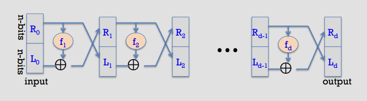
#### Block cipher constructions: Feistel network
|
|
||||||
|
|
||||||
Forward network:
|
|
||||||
|
|
||||||
|
|
||||||
|
|
||||||
- Forward (round $i$): given $(L_{i-1}, R_{i-1}) \in \{0,1\}^n \times \{0,1\}^n$,
|
|
||||||
- $L_i = R_{i-1}$
|
|
||||||
- $R_i = L_{i-1} \oplus f_i(R_{i-1})$
|
|
||||||
|
|
||||||
- Proof (construct the inverse):
|
|
||||||
- Suppose we are given the output of round $i$, namely $(L_i, R_i)$.
|
|
||||||
- Recover the previous right half immediately:
|
|
||||||
- $R_{i-1} = L_i$
|
|
||||||
- Then recover the previous left half by undoing the XOR:
|
|
||||||
- $L_{i-1} = R_i \oplus f_i(R_{i-1}) = R_i \oplus f_i(L_i)$
|
|
||||||
- Therefore each round map is invertible, with inverse transformation:
|
|
||||||
- $R_{i-1} = L_i$
|
|
||||||
- $L_{i-1} = f_i(L_i) \oplus R_i$
|
|
||||||
- Applying this inverse for $i=d,d-1,\ldots,1$ recovers $(L_0,R_0)$ from $(L_d,R_d)$, so the whole Feistel network $F$ is invertible.
|
|
||||||
|
|
||||||
- Notation sketch (each wire is $n$ bits):
|
|
||||||
- Input: $(L_0, R_0)$
|
|
||||||
- Rounds:
|
|
||||||
- $L_1 = R_0,\ \ R_1 = L_0 \oplus f_1(R_0)$
|
|
||||||
- $L_2 = R_1,\ \ R_2 = L_1 \oplus f_2(R_1)$
|
|
||||||
- $\cdots$
|
|
||||||
- $L_d = R_{d-1},\ \ R_d = L_{d-1} \oplus f_d(R_{d-1})$
|
|
||||||
- Output: $(L_d, R_d)$
|
|
||||||
|
|
||||||
#### Block ciphers: block modes: ECB
|
|
||||||
|
|
||||||
New attacker model for multi-use keys (e.g. multiple blocks): CPA (Chosen Plaintext)-capable, not just CT-only
|
|
||||||
|
|
||||||
- Attacker sees many PT/CT pairs for same key
|
|
||||||
- Conservative model: attacker submits arbitrary PT (hence "C"PA)
|
|
||||||
- Cipher goal: maintain semantic security against CPA
|
|
||||||
|
|
||||||
#### CPA indistinguishability game
|
|
||||||
|
|
||||||
- Updated adversarial game for a CPA attacker:
|
|
||||||
- Let $E = (E, D)$ be a cipher defined over $(K, M, C)$. For $b \in \{0,1\}$ define $\operatorname{EXP}(b)$ as:
|
|
||||||
|
|
||||||
- Experiment $\operatorname{EXP}(b)$:
|
|
||||||
- Challenger samples $k \leftarrow K$.
|
|
||||||
- For each query $i = 1,\ldots,q$:
|
|
||||||
- Adversary outputs messages $m_{i,0}, m_{i,1} \in M$ such that $|m_{i,0}| = |m_{i,1}|$.
|
|
||||||
- Challenger returns $c_i \leftarrow E(k, m_{i,b})$.
|
|
||||||
|
|
||||||
- Encryption-oracle access (CPA):
|
|
||||||
- If the adversary wants $c = E(k, m)$, it queries with $m_{j,0} = m_{j,1} = m$ (so the response is $E(k,m)$ regardless of $b$).
|
|
||||||
|
|
||||||
#### Semantic security under CPA
|
|
||||||
|
|
||||||
- Def: $E$ is semantically secure under CPA if for all "efficient" adversaries $A$,
|
|
||||||
- $\operatorname{Adv}^{\operatorname{CPA}}[A,E] = \left|\Pr[\operatorname{EXP}(0)=1] - \Pr[\operatorname{EXP}(1)=1]\right|$
|
|
||||||
- is negligible.
|
|
||||||
|
|
||||||
### Summary for symmetric encrption
|
|
||||||
|
|
||||||
1. Stream ciphers
|
|
||||||
- Rely on secure PRG
|
|
||||||
- No key re-use
|
|
||||||
- Fast, low-mem, less robust
|
|
||||||
2. Block ciphers
|
|
||||||
- Rely on secure PRP
|
|
||||||
- Allow key re-use (usually only across blocks, not sessions)
|
|
||||||
- Provide authenticated encryption in some modes (e.g. GCM)
|
|
||||||
- Slower, higher-mem, more robust
|
|
||||||
- Used in practice for most crypto tasks (including secure network channels)
|
|
||||||
|
|
||||||
## Hash functions
|
|
||||||
|
|
||||||
### Hash function security properties
|
|
||||||
|
|
||||||
- Given a function $h:X \to Y$, we say that $h$ is:
|
|
||||||
|
|
||||||
- 1. Preimage resistant (one-way) if:
|
|
||||||
- given $y \in Y$ it is computationally infeasible to find a value $x \in X$ s.t. $h(x) = y$
|
|
||||||
|
|
||||||
- 2. 2nd preimage resistant (weak collision resistant) if:
|
|
||||||
- given a specific $x \in X$ it is computationally infeasible to find a value $x' \in X$ s.t. $x' \ne x$ and $h(x') = h(x)$
|
|
||||||
|
|
||||||
- 3. Collision resistant (strong collision resistant) if:
|
|
||||||
- it is computationally infeasible to find any two distinct values $x', x \in X$ s.t. $h(x') = h(x)$
|
|
||||||
|
|
||||||
### Collision resistance: adversarial definition
|
|
||||||
|
|
||||||
- Let $H: M \to T$ be a hash function ($|M| \gg |T|$).
|
|
||||||
- A function $H$ is collision resistant if for all (explicit) "efficient" algorithms $A$,
|
|
||||||
- $\operatorname{Adv}^{\operatorname{CR}}[A,H] = Pr[$A outputs a collision for $H$ $]$
|
|
||||||
- is negligible
|
|
||||||
|
|
||||||
### Hash function integrity applications
|
|
||||||
|
|
||||||
1. Delayed knowledge verification
|
|
||||||
2. Password storage
|
|
||||||
3. Trusted timestamping / blockchains
|
|
||||||
4. Integrity check on software
|
|
||||||
|
|
||||||
#### File integrity with secure read-only space
|
|
||||||
|
|
||||||
- When user downloads package, can verify that contents are valid
|
|
||||||
- $H$ collision resistant $\Rightarrow$ attacker cannot modify package without detection
|
|
||||||
- No encryption needed (public verifiability) if publisher has secure read-only space (e.g. trusted website, social media account)
|
|
||||||
|
|
||||||
#### Symmetric-crypto message authentication
|
|
||||||
|
|
||||||
- Context: Assume no secure RO space (insecure channel only)
|
|
||||||
- Need means of message authentication
|
|
||||||
- Idea: add tag to message
|
|
||||||
- System: Message Authentication Code (MAC)
|
|
||||||
- Def: a MAC $I=(S,V)$ defined over $(K,M,T)$ is a pair of algorithms:
|
|
||||||
- $S(k,m)$ outputs $t \in T$ // "Sign"
|
|
||||||
- $V(k,m,t)$ outputs `yes' or `no' // "Verify"
|
|
||||||
|
|
||||||
- Symmetric-crypto message authentication:
|
|
||||||
- Alice and Bob share secret key $k$
|
|
||||||
- Generate tag: $\text{tag} \leftarrow S(k,m)$
|
|
||||||
- Verify tag: $V(k,m,\text{tag}) = \texttt{yes}?$
|
|
||||||
|
|
||||||
#### MAC security model
|
|
||||||
|
|
||||||
- For a MAC $I=(S,V)$ and adversary $A$, define a MAC game as:
|
|
||||||
- Def: $I=(S,V)$ is a secure MAC if for all "efficient" $A$,
|
|
||||||
- $\operatorname{Adv}^{\operatorname{MAC}}[A,I] = \Pr[\text{Chal. outputs }1]$
|
|
||||||
- is negligible
|
|
||||||
|
|
||||||
- MAC game (sketch):
|
|
||||||
- Challenger samples $k \leftarrow K$
|
|
||||||
- Adversary makes queries $m_1,\ldots,m_q \in M$
|
|
||||||
- For each $i$, challenger returns $t_i \leftarrow S(k,m_i)$
|
|
||||||
- Adversary outputs a candidate forgery $(m,t)$
|
|
||||||
- Challenger outputs $b=1$ if:
|
|
||||||
- $V(k,m,t)=\texttt{yes}$ and
|
|
||||||
- $(m,t) \notin \{(m_1,t_1),\ldots,(m_q,t_q)\}$
|
|
||||||
- Otherwise challenger outputs $b=0$
|
|
||||||
|
|
||||||
- MAC security example: secure PRF not sufficient
|
|
||||||
- Suppose $F: K \times X \to Y$ is a secure PRF with $Y=\{0,1\}^{10}$.
|
|
||||||
- Is the derived MAC $I_F$ a secure MAC system?
|
|
||||||
- No: tags are too short, anyone can guess the tag for any message
|
|
||||||
|
|
||||||
#### MACs from PRFs: sufficient security condition
|
|
||||||
|
|
||||||
- Thm: If $F: K \times X \to Y$ is a secure PRF and $1/|Y|$ is negligible (i.e. $|Y|$ is large), then $I_F$ is a secure MAC.
|
|
||||||
- In particular, for every efficient MAC adversary $A$ attacking $I_F$, there exists an efficient PRF adversary $B$ attacking $F$ such that:
|
|
||||||
- $\operatorname{Adv}^{\operatorname{MAC}}[A, I_F] \le \operatorname{Adv}^{\operatorname{PRF}}[B, F] + 1/|Y|$
|
|
||||||
- Therefore $I_F$ is secure as long as $|Y|$ is large, e.g. $|Y| = 2^{80}$.
|
|
||||||
|
|
||||||
#### MACs from collision resistance
|
|
||||||
|
|
||||||
- Let $I=(S,V)$ be a MAC for short messages over $(K,M,T)$ (e.g. AES).
|
|
||||||
- Let $H: M_{\text{big}} \to M$.
|
|
||||||
- Def: $I_{\text{big}}=(S_{\text{big}},V_{\text{big}})$ over $(K,M_{\text{big}},T)$ as:
|
|
||||||
- $S_{\text{big}}(k,m) = S(k, H(m))$
|
|
||||||
- $V_{\text{big}}(k,m,t) = V(k, H(m), t)$
|
|
||||||
- Thm: If $I$ is a secure MAC and $H$ is collision resistant, then $I_{\text{big}}$ is a secure MAC.
|
|
||||||
- Example: $S(k,m) = \operatorname{AES2\text{-}block\text{-}cbc}(k, \operatorname{SHA\text{-}256}(m))$ is a secure MAC.
|
|
||||||
|
|
||||||
#### Using HMACs for confidentiality + integrity
|
|
||||||
|
|
||||||
- Confidentiality:
|
|
||||||
- Semantic security under a CPA
|
|
||||||
- Encryption secure against eavesdropping only
|
|
||||||
- Integrity:
|
|
||||||
- Existential unforgeability under a CPA
|
|
||||||
- CBC-MAC, HMAC
|
|
||||||
- Hash functions
|
|
||||||
- Confidentiality + integrity:
|
|
||||||
- CCA security
|
|
||||||
- Secure against tampering
|
|
||||||
- Method: Authenticated Encryption (AE)
|
|
||||||
- Encryption + MAC, in correct form
|
|
||||||
|
|
||||||
#### Authenticated Encryption: security defs
|
|
||||||
|
|
||||||
- An authenticated encryption system $(E,D)$ is a cipher where:
|
|
||||||
- $E: K \times M \times N \to C$
|
|
||||||
- $D: K \times C \times N \to M \cup$ cipher text rejected
|
|
||||||
- Security: the system must provide
|
|
||||||
- semantic security under a CPA attack, and
|
|
||||||
- ciphertext integrity: attacker cannot create new ciphertexts that decrypt properly
|
|
||||||
|
|
||||||
#### Ciphertext integrity
|
|
||||||
|
|
||||||
- Let $(E,D)$ be a cipher with message space $M$.
|
|
||||||
- Def: $(E,D)$ has ciphertext integrity if for all "efficient" $A$,
|
|
||||||
- $\operatorname{Adv}^{\operatorname{CI}}[A,E] = \Pr[\text{Chal. outputs }1]$
|
|
||||||
- is negligible
|
|
||||||
|
|
||||||
- Security model: ciphertext integrity (sketch):
|
|
||||||
- Challenger samples $k \leftarrow K$
|
|
||||||
- Adversary makes encryption queries $m_1,\ldots,m_q \in M$
|
|
||||||
- For each $i$, challenger returns $c_i \leftarrow E(k,m_i)$
|
|
||||||
- Adversary outputs a ciphertext $c$
|
|
||||||
- Challenger outputs $b=1$ if:
|
|
||||||
- $D(k,c) \ne \bot$ and
|
|
||||||
- $c \notin \{c_1,\ldots,c_q\}$
|
|
||||||
- Otherwise challenger outputs $b=0$
|
|
||||||
|
|
||||||
#### Authenticated encryption implies CCA security
|
|
||||||
|
|
||||||
- Thm: Let $(E,D)$ be a cipher that provides AE. Then $(E,D)$ is CCA secure.
|
|
||||||
- In particular, for any $q$-query efficient adversary $A$, there exist efficient $B_1,B_2$ such that:
|
|
||||||
- $\operatorname{Adv}^{\operatorname{CCA}}[A,E] \le 2q \cdot \operatorname{Adv}^{\operatorname{CI}}[B_1,E] + \operatorname{Adv}^{\operatorname{CPA}}[B_2,E]$
|
|
||||||
- Interpretation: CCA advantage is $\le O(\text{CT-integrity advantage}) + \text{CPA advantage}$.
|
|
||||||
|
|
||||||
- AE implication: authenticity
|
|
||||||
- Attacker cannot fool Bob into thinking a message was sent from Alice
|
|
||||||
- If attacker cannot create a valid ciphertext $c \notin \{c_1,\ldots,c_q\}$, then whenever $D(k,c) \ne \bot$ Bob knows the message is from someone who knows $k$ (but it could be a replay)
|
|
||||||
|
|
||||||
- DS construction example: signing a certificate
|
|
||||||
|
|
||||||
### Comparison: integrity/authentication approaches
|
|
||||||
|
|
||||||
- 1) Collision resistant hashing: need a read-only public space
|
|
||||||
- Allows public verification if the hash is published in a small read-only public space
|
|
||||||
- 2) MACs: must compute a new MAC for every client/user
|
|
||||||
- Must manage a long-term secret key per user to verify MACs (depending on application)
|
|
||||||
- Typically useful when one party signs, one verifies
|
|
||||||
- 3) Digital signatures: must manage a long-term secret key
|
|
||||||
- E.g. vendor's signature on software is shipped with software
|
|
||||||
- Allows software to be downloaded from an untrusted distribution site
|
|
||||||
- Public-key verification/rejection works, provided public key distribution is trustworthy
|
|
||||||
- Typically useful when one party signs, many verify
|
|
||||||
|
|
||||||
## Asymmetric key cryptography
|
|
||||||
|
|
||||||
### Asymmetric crypto overview
|
|
||||||
|
|
||||||
- Parties: sender, recipient, attacker (eavesdropping)
|
|
||||||
- Goal: sender encrypts a plaintext to a ciphertext using a public key; recipient decrypts using a private key.
|
|
||||||
|
|
||||||
#### Public-key encryption system
|
|
||||||
|
|
||||||
- Def: a public-key encryption system is a triple of algorithms $(G, E, D)$:
|
|
||||||
- $G()$: randomized algorithm that outputs a key pair $(pk, sk)$
|
|
||||||
- $E(pk, m)$: randomized algorithm that takes $m \in M$ and outputs $c \in C$
|
|
||||||
- $D(sk, c)$: deterministic algorithm that takes $c \in C$ and outputs $m \in M$ or $\bot$
|
|
||||||
- Consistency: for all $(pk, sk)$ output by $G$, for all $m \in M$,
|
|
||||||
- $D(sk, E(pk, m)) = m$
|
|
||||||
|
|
||||||
#### Trapdoor function
|
|
||||||
|
|
||||||
- Def: a trapdoor function $X \to Y$ is a triple of efficient algorithms $(G, F, F^{-1})$:
|
|
||||||
- $G()$: randomized algorithm that outputs a key pair $(pk, sk)$
|
|
||||||
- $F(pk, \cdot)$: deterministic algorithm that defines a function $X \to Y$
|
|
||||||
- $F^{-1}(sk, \cdot)$: defines a function $Y \to X$ that inverts $F(pk, \cdot)$
|
|
||||||
- More precisely: for all $(pk, sk)$ output by $G$, for all $x \in X$,
|
|
||||||
- $F^{-1}(sk, F(pk, x)) = x$
|
|
||||||
|
|
||||||
#### Symmetric vs. asymmetric security: attacker models
|
|
||||||
|
|
||||||
- Symmetric ciphers: two security notions for a passive attacker
|
|
||||||
- One-time security (stream ciphers: ciphertext-only)
|
|
||||||
- Many-time security (block ciphers: CPA)
|
|
||||||
- One-time security $\Rightarrow$ many-time security
|
|
||||||
- Example: ECB mode is one-time secure but not many-time secure
|
|
||||||
- Public-key encryption: single notion for a passive attacker
|
|
||||||
- Attacker can encrypt by themselves using the public key
|
|
||||||
- Therefore one-time security $\Rightarrow$ many-time security (CPA)
|
|
||||||
- Implication: public-key encryption must be randomized
|
|
||||||
- Analogous to secure block modes for block ciphers
|
|
||||||
|
|
||||||
### Semantic security of asymmetric crypto (IND-CPA)
|
|
||||||
|
|
||||||
#### IND-CPA game for public-key encryption
|
|
||||||
|
|
||||||
- For $b \in \{0,1\}$ define experiments $\operatorname{EXP}(0)$ and $\operatorname{EXP}(1)$:
|
|
||||||
|
|
||||||
- Experiment $\operatorname{EXP}(b)$:
|
|
||||||
- Challenger runs $(pk, sk) \leftarrow G()$
|
|
||||||
- Challenger sends $pk$ to adversary $A$
|
|
||||||
- Adversary outputs $m_0, m_1 \in M$ such that $|m_0| = |m_1|$
|
|
||||||
- Challenger returns $c \leftarrow E(pk, m_b)$
|
|
||||||
- Adversary outputs a bit $b' \in \{0,1\}$ (often modeled as outputting 1 if it "guesses $b=1$")
|
|
||||||
|
|
||||||
#### Semantic security (IND-CPA)
|
|
||||||
|
|
||||||
- Def: $E = (G, E, D)$ is semantically secure (a.k.a. IND-CPA) if for all efficient adversaries $A$,
|
|
||||||
- $\operatorname{Adv}^{\operatorname{SS}}[A, E] = \left|\Pr[\operatorname{EXP}(0)=1] - \Pr[\operatorname{EXP}(1)=1]\right|$
|
|
||||||
- is negligible
|
|
||||||
- Note: inherently multiple-round because the attacker can always encrypt on their own using $pk$ (CPA power is "built in").
|
|
||||||
|
|
||||||
### RSA cryptosystem: overview
|
|
||||||
|
|
||||||
- Setup:
|
|
||||||
- $n = pq$, with $p$ and $q$ primes
|
|
||||||
- Choose $e$ relatively prime to $\phi(n) = (p-1)(q-1)$
|
|
||||||
- Choose $d$ as the inverse of $e$ in $\mathbb{Z}_{\phi(n)}$
|
|
||||||
- Keys:
|
|
||||||
- Public key: $K_E = (n, e)$
|
|
||||||
- Private key: $K_D = d$
|
|
||||||
- Encryption:
|
|
||||||
- Plaintext $M \in \mathbb{Z}_n$
|
|
||||||
- $C = M^e \bmod n$
|
|
||||||
- Decryption:
|
|
||||||
- $M = C^d \bmod n$
|
|
||||||
|
|
||||||
- Example:
|
|
||||||
- Setup:
|
|
||||||
- $p = 7$, $q = 17$
|
|
||||||
- $n = 7 \cdot 17 = 119$
|
|
||||||
- $\phi(n) = 6 \cdot 16 = 96$
|
|
||||||
- $e = 5$
|
|
||||||
- $d = 77$
|
|
||||||
- Keys:
|
|
||||||
- public key: $(119, 5)$
|
|
||||||
- private key: $77$
|
|
||||||
- Encryption:
|
|
||||||
- $M = 19$
|
|
||||||
- $C = 19^5 \bmod 119 = 66$
|
|
||||||
- Decryption:
|
|
||||||
- $M = 66^{77} \bmod 119 = 19$
|
|
||||||
|
|
||||||
- Security intuition:
|
|
||||||
- To invert RSA without $d$, attacker must compute $x$ from $c = x^e \pmod n$.
|
|
||||||
- Best known approach:
|
|
||||||
- Step 1: factor $n$ (hard)
|
|
||||||
- Step 2: compute $e$-th roots modulo $p$ and $q$ (easy once factored)
|
|
||||||
- Notes (as commonly stated in lectures):
|
|
||||||
- 1024-bit RSA is within reach; 2048-bit is recommended usage
|
|
||||||
|
|
||||||
### Diffie-Hellman key exchange (informal)
|
|
||||||
|
|
||||||
- Fix a large prime $p$ (e.g., 2000 bits)
|
|
||||||
- Fix an integer $g \in \{1,\ldots,p\}$
|
|
||||||
|
|
||||||
- Protocol:
|
|
||||||
- Alice chooses random $a \in \{1,\ldots,p-1\}$ and sends $A = g^a \bmod p$
|
|
||||||
- Bob chooses random $b \in \{1,\ldots,p-1\}$ and sends $B = g^b \bmod p$
|
|
||||||
- Shared key:
|
|
||||||
- Alice computes $k_{AB} = B^a \bmod p = g^{ab} \bmod p$
|
|
||||||
- Bob computes $k_{AB} = A^b \bmod p = g^{ab} \bmod p$
|
|
||||||
|
|
||||||
- Hardness assumptions:
|
|
||||||
- Discrete log problem: given $p, g, y = g^x \bmod p$, find $x$
|
|
||||||
- Diffie-Hellman function: $\operatorname{DH}_g(g^a, g^b) = g^{ab} \bmod p$
|
|
||||||
|
|
||||||
#### Diffie-Hellman: security notes
|
|
||||||
|
|
||||||
- As described, the protocol is insecure against active attacks:
|
|
||||||
- A man-in-the-middle (MiTM) can insert themselves and create 2 separate secure sessions
|
|
||||||
- Fix idea: need a way to bind identity to a public key
|
|
||||||
- In practice: web of trust (e.g., GPG) or Public Key Infrastructure (PKI)
|
|
||||||
|
|
||||||
### Implementing trapdoor functions securely
|
|
||||||
|
|
||||||
- Never encrypt by applying $F$ directly to plaintext:
|
|
||||||
- Deterministic: cannot be semantically secure
|
|
||||||
- Many attacks exist for concrete TDFs
|
|
||||||
- Same plaintext blocks yield same ciphertext blocks
|
|
||||||
|
|
||||||
- Naive (insecure) sketch:
|
|
||||||
- $E(pk, m)$: output $c \leftarrow F(pk, m)$
|
|
||||||
- $D(sk, c)$: output $F^{-1}(sk, c)$
|
|
||||||
|
|
||||||
### Public-key encryption from TDFs
|
|
||||||
|
|
||||||
- Components:
|
|
||||||
- $(G, F, F^{-1})$: secure TDF $X \to Y$
|
|
||||||
- $(E_s, D_s)$: symmetric authenticated encryption over $(K, M, C)$
|
|
||||||
- $H: X \to K$: a hash function
|
|
||||||
|
|
||||||
- Construction of $(G, E, D)$ (with $G$ same as in the TDF):
|
|
||||||
- $E(pk, m)$:
|
|
||||||
- sample $x \leftarrow X$, compute $y \leftarrow F(pk, x)$
|
|
||||||
- derive $k \leftarrow H(x)$, compute $c \leftarrow E_s(k, m)$
|
|
||||||
- output $(y, c)$
|
|
||||||
- $D(sk, (y, c))$:
|
|
||||||
- compute $x \leftarrow F^{-1}(sk, y)$
|
|
||||||
- derive $k \leftarrow H(x)$, compute $m \leftarrow D_s(k, c)$
|
|
||||||
- output $m$
|
|
||||||
|
|
||||||
- Visual intuition:
|
|
||||||
- header: $y = F(pk, x)$
|
|
||||||
- body: $c = E_s(H(x), m)$
|
|
||||||
|
|
||||||
- Security theorem (lecture-style statement):
|
|
||||||
- If $(G, F, F^{-1})$ is a secure TDF, $(E_s, D_s)$ provides authenticated encryption, and $H$ is modeled as a random oracle, then $(G, E, D)$ is CCA-secure in the random oracle model (often denoted CCA-RO).
|
|
||||||
- Extension exists to reach full CCA (outside the RO idealization).
|
|
||||||
|
|
||||||
### Wrapup: symmetric vs. asymmetric systems
|
|
||||||
|
|
||||||
- Symmetric: faster, but key distribution is hard
|
|
||||||
- Asymmetric: slower, but key distribution/management is easier
|
|
||||||
- Application: secure web sessions (e.g., online shopping)
|
|
||||||
- Use symmetric-key encrypted sessions for bulk traffic
|
|
||||||
- Exchange symmetric keys using an asymmetric scheme
|
|
||||||
- Authenticate public keys (PKI or web of trust)
|
|
||||||
|
|
||||||
### Key exchange: summary
|
|
||||||
|
|
||||||
- Symmetric-key encryption challenges:
|
|
||||||
- Key storage: one per user pair, $O(n^2)$ total for $n$ users
|
|
||||||
- Key exchange: how to do it over a non-secure channel?
|
|
||||||
|
|
||||||
- Possible solutions:
|
|
||||||
|
|
||||||
- 1) Trusted Third Party (TTP)
|
|
||||||
- All users establish separate secret keys with the TTP
|
|
||||||
- TTP helps manage user-user keys (storage and secure channel)
|
|
||||||
- Applicability:
|
|
||||||
- Works for local domains
|
|
||||||
- Popular implementation: Kerberos for Single Sign On (SSO)
|
|
||||||
- Challenges:
|
|
||||||
- Scale: central authentication server is not suitable for the entire Internet
|
|
||||||
- Latency: requires online response from central server for every user-user session
|
|
||||||
|
|
||||||
- 2) Public/private keys with certificates
|
|
||||||
- All users have a single stable public key (helps with key storage and exchange)
|
|
||||||
- Users exchange per-session symmetric keys via a secure channel using public/private keys
|
|
||||||
- Trusting public keys: binding is validated by a third-party authority (Certificate Authority, CA)
|
|
||||||
- Why better than TTP? CAs can validate statically by issuing certificates, then be uninvolved
|
|
||||||
- CA/certificate process covered in a future lecture
|
|
||||||
|
|
||||||
## Appendix for additional algorithms and methods
|
|
||||||
|
|
||||||
### Feistel network (used by several items below)
|
|
||||||
|
|
||||||
A **Feistel network** splits a block into left/right halves and iterates rounds of the form $(L_{i+1},R_{i+1})=(R_i, L_i\oplus F(R_i,K_i))$, so decryption reuses the same structure with subkeys in reverse order.
|
|
||||||
|
|
||||||
Feistel-based here: **DES, 3DES, CAMELLIA, SEED, GOST 28147-89 (and thus GOST89MAC uses a Feistel block cipher internally).**
|
|
||||||
|
|
||||||
### Key exchange and authentication selectors (not symmetric encryption, not MAC)
|
|
||||||
|
|
||||||
These describe *how keys are negotiated- and/or *how the peer is authenticated*, not whether payload is a block/stream cipher.
|
|
||||||
|
|
||||||
#### RSA / DH / ECDH families
|
|
||||||
|
|
||||||
- **kRSA, RSA** — (key exchange) the premaster secret is sent encrypted under the server’s RSA public key (classic TLS RSA KX).
|
|
||||||
- **aRSA, aECDSA, aDSS, aGOST, aGOST01** — (authentication) the server identity is proven via a certificate signature scheme (RSA / ECDSA / DSA / GOST).
|
|
||||||
- **kDHr, kDHd, kDH** — (key exchange) *static- DH key agreement using DH certificates (obsolete/removed in newer OpenSSL).
|
|
||||||
- **kDHE, kEDH, DH / DHE, EDH / ECDHE, EECDH / kEECDH, kECDHE, ECDH** — (key exchange) *ephemeral- (EC)DH derives a fresh shared secret each handshake; "authenticated" variants bind it to a cert/signature.
|
|
||||||
- **aDH** — (authentication selector) indicates DH-authenticated suites (DH certs; also removed in newer OpenSSL).
|
|
||||||
|
|
||||||
#### PSK family
|
|
||||||
|
|
||||||
- **PSK** — (keying model) uses a pre-shared secret as the authentication/secret basis.
|
|
||||||
- **kPSK, kECDHEPSK, kDHEPSK, kRSAPSK** — (key exchange) PSK combined with (EC)DHE or RSA to derive/transport session keys.
|
|
||||||
- **aPSK** — (authentication) PSK itself authenticates endpoints (except RSA_PSK where cert auth may be involved).
|
|
||||||
|
|
||||||
---
|
|
||||||
|
|
||||||
### Symmetric encryption / AEAD (this is where "block vs stream" applies)
|
|
||||||
|
|
||||||
#### AES family
|
|
||||||
|
|
||||||
- **AES128 / AES256 / AES** — **encryption/decryption**; **block cipher**; core algorithm: AES is an SPN (substitution–permutation network) of repeated SubBytes/ShiftRows/MixColumns/AddRoundKey rounds.
|
|
||||||
- **AES-GCM** — **both encryption + message authentication (AEAD)**; **both** (AES block cipher used in counter mode + auth); core algorithm: encrypt with AES-CTR and authenticate with GHASH over ciphertext/AAD to produce a tag.
|
|
||||||
- **AES-ECB**: Functionality is encryption/decryption (confidentiality only) using a block cipher mode; core algorithm encrypts each 128-bit plaintext block independently under the same key, which deterministically leaks patterns because equal plaintext blocks map to equal ciphertext blocks.
|
|
||||||
- **AES-CBC**: Functionality is encryption/decryption (confidentiality only) using a block cipher mode; core algorithm XORs each plaintext block with the previous ciphertext block (starting from a fresh unpredictable IV) before AES-encrypting, which hides repetitions but requires correct IV handling and padding for non-multiple-of-block messages.
|
|
||||||
- **AES-OFB** — **encryption**; both (stream-like); repeatedly AES-encrypts an internal state to generate a keystream and XORs it with plaintext, where the state evolves independently of the plaintext/ciphertext.
|
|
||||||
- **AESCCM / AESCCM8** — **both encryption + message authentication (AEAD)**; **both**; core algorithm: compute CBC-MAC then encrypt with CTR mode, with 16-byte vs 8-byte tag length variants.
|
|
||||||
|
|
||||||
#### ARIA family
|
|
||||||
|
|
||||||
- **ARIA128 / ARIA256 / ARIA** — **encryption/decryption**; **block cipher**; core algorithm: ARIA is an SPN-style block cipher with byte-wise substitutions and diffusion layers across rounds.
|
|
||||||
|
|
||||||
#### CAMELLIA family
|
|
||||||
|
|
||||||
- **CAMELLIA128 / CAMELLIA256 / CAMELLIA** — **encryption/decryption**; **block cipher**; core algorithm: Camellia is a **Feistel network** with round functions plus extra FL/FL$^{-1}$ layers for nonlinearity and diffusion. *(Feistel: yes)*
|
|
||||||
|
|
||||||
#### ChaCha20
|
|
||||||
|
|
||||||
- **CHACHA20** — **encryption/decryption**; **stream cipher**; core algorithm: ChaCha20 generates a keystream via repeated ARX (add-rotate-xor) quarter-rounds on a 512-bit state and XORs it with plaintext.
|
|
||||||
|
|
||||||
#### DES / 3DES
|
|
||||||
|
|
||||||
- **DES** — **encryption/decryption**; **block cipher**; core algorithm: DES is a 16-round **Feistel network** using expansion, S-boxes, and permutations. *(Feistel: yes)*
|
|
||||||
- **3DES** — **encryption/decryption**; **block cipher**; core algorithm: applies DES three times (EDE or EEE) to increase effective security while retaining the **Feistel** DES core. *(Feistel: yes)*
|
|
||||||
|
|
||||||
#### RC4
|
|
||||||
|
|
||||||
- **RC4** — **encryption/decryption**; **stream cipher**; core algorithm: maintains a 256-byte permutation and produces a keystream byte-by-byte that is XORed with plaintext.
|
|
||||||
|
|
||||||
#### RC2 / IDEA / SEED
|
|
||||||
|
|
||||||
- **RC2** — **encryption/decryption**; **block cipher**; core algorithm: mixes key-dependent operations (adds, XORs, rotates) across rounds with "mix" and "mash" steps (not Feistel).
|
|
||||||
- **IDEA** — **encryption/decryption**; **block cipher**; core algorithm: combines modular addition, modular multiplication, and XOR in a Lai–Massey-like structure to achieve diffusion/nonlinearity (not Feistel).
|
|
||||||
- **SEED** — **encryption/decryption**; **block cipher**; core algorithm: a 16-round **Feistel network** with nonlinear S-box-based round functions. *(Feistel: yes)*
|
|
||||||
|
|
||||||
---
|
|
||||||
|
|
||||||
### Hash / MAC / digest selectors (message authentication side)
|
|
||||||
|
|
||||||
These are not "ciphers" but are used for integrity/authentication (often as HMAC, PRF, signatures).
|
|
||||||
|
|
||||||
- **MD5** — **message authentication component** (typically via HMAC, historically); **cipher method: N/A**; core algorithm: iterated Merkle–Damgård hash compressing 512-bit blocks into a 128-bit digest (now considered broken for collision resistance).
|
|
||||||
- **SHA1, SHA** — **message authentication component** (typically HMAC-SHA1 historically); **N/A**; core algorithm: Merkle–Damgård hash producing 160-bit output via 80-step compression (collisions known).
|
|
||||||
- **SHA256 / SHA384** — **message authentication component** (HMAC / TLS PRF / signatures); **N/A**; core algorithm: SHA-2 family Merkle–Damgård hashes with different word sizes/output lengths (256-bit vs 384-bit).
|
|
||||||
- **GOST94** — **message authentication component** (HMAC based on GOST R 34.11-94); **N/A**; core algorithm: builds an HMAC tag by hashing inner/outer padded key with the message using the GOST hash.
|
|
||||||
- **GOST89MAC** — **message authentication**; **block-cipher-based MAC (so "block" internally)**; core algorithm: computes a MAC using the GOST 28147-89 block cipher in a MAC mode (cipher-based chaining). *(Feistel internally via GOST 28147-89)*
|
|
||||||
|
|
||||||
> Latest version of cheatsheet distilled from this note.
|
|
||||||
@@ -1,112 +0,0 @@
|
|||||||
# CSE4303 Introduction to Computer Security (Lecture 1)
|
|
||||||
|
|
||||||
## Course introduction and security fundamentals
|
|
||||||
|
|
||||||
### Computer Security Ethics
|
|
||||||
|
|
||||||
In this course, you will learn about tools and techniques that cna be used to violate privacy, cause harm, or undermine trust.
|
|
||||||
|
|
||||||
"The difference between a professional and a threat actor is not the technique -- it's intent, restraint, and accountability." -- ChatGPT
|
|
||||||
|
|
||||||
Intent:
|
|
||||||
|
|
||||||
Am I doing this for good or for bad?
|
|
||||||
|
|
||||||
Restraint:
|
|
||||||
|
|
||||||
Just because I can, should I?
|
|
||||||
|
|
||||||
Accountability:
|
|
||||||
|
|
||||||
Am I willing to take responsibility for my
|
|
||||||
actions, even when my name isn’t on them?
|
|
||||||
If my actions cause unintended harm, are my
|
|
||||||
actions defensible?
|
|
||||||
|
|
||||||
**Strive to be the good guy**
|
|
||||||
|
|
||||||
> [!WARNING]
|
|
||||||
>
|
|
||||||
> Disclaimer: If you choose to experiment on systems you do not own, do not have permission to test, or engage in illegal activity, that is a personal choice—not a course activity. In those cases, you should not expect support, protection, or advocacy from the instructional staff or the university.
|
|
||||||
|
|
||||||
What is there to gain?
|
|
||||||
|
|
||||||
- Access to systems
|
|
||||||
|
|
||||||
Trust and reputation are critical in cybersecurity. If you do not have a strong reputation as a professional, no one will trust you with access to their systems!
|
|
||||||
|
|
||||||
### Course learning objectives
|
|
||||||
|
|
||||||
1. Understand principles of security analysis
|
|
||||||
2. Explain key security concepts such as confidentiality
|
|
||||||
3. Explain the root causes of current security problems
|
|
||||||
4. Produce clear and concise descriptions of security problems on real world systems
|
|
||||||
5. Analyze systems for potential vulnerabilities
|
|
||||||
|
|
||||||
Slides contain material from Computer Security lectures taught by
|
|
||||||
|
|
||||||
- Prof. Dan Boneh from Stanford
|
|
||||||
- Prof. Wenke Lee from Georgia Tech
|
|
||||||
- Prof. Wenliang (Kevin) Du from Syracuse
|
|
||||||
- Profs. Zhang and Cole
|
|
||||||
|
|
||||||
These sources will be used for slides throughout the course
|
|
||||||
|
|
||||||
## Defining security
|
|
||||||
|
|
||||||
How would you define security?
|
|
||||||
|
|
||||||
- informal: protecting something (information, system) against stealing, changing, destroying, forging etc.
|
|
||||||
- Slightly more formal:
|
|
||||||
- Ensuring that assets
|
|
||||||
- Can be accessed by those with authority to do so
|
|
||||||
- Cannot be accessed by those without it
|
|
||||||
|
|
||||||
The security of a system, application, or protocol is always relative to
|
|
||||||
|
|
||||||
- A set of desired properties
|
|
||||||
- anonymity, confidentiality, authenticity, and more
|
|
||||||
- An adversary with specific capabilities ("threat model")
|
|
||||||
- I put the pizza on top of the fridge so the dog couldn’t reach it. I forgot about the cat
|
|
||||||
|
|
||||||
## Key security concepts
|
|
||||||
|
|
||||||
Confidentiality: no unauthorized disclosure of information
|
|
||||||
|
|
||||||
- Tools to achieve it
|
|
||||||
- Encryption
|
|
||||||
- Access control
|
|
||||||
- Authentication (passwords, biometrics, etc.)
|
|
||||||
|
|
||||||
Integrity: information is not altered from original content in unauthorized way
|
|
||||||
|
|
||||||
- Tools to achieve it:
|
|
||||||
- Backups (hot and cold, on-site and off-site)
|
|
||||||
- Checksums and hash functions
|
|
||||||
|
|
||||||
Availability: information and resources are accessible to those authorized to have it
|
|
||||||
|
|
||||||
- Threats:
|
|
||||||
- Resource (e.g. website): Denial of Service (DoS or DDoS) attack
|
|
||||||
- Example: Murai botnet makes popular websites unavailable (2016)
|
|
||||||
- Video: Murai in 100 seconds
|
|
||||||
- Example: DDoS attacks increase in work-from-home COVID-19environment
|
|
||||||
- Complexity attacks
|
|
||||||
- Data: ransomware
|
|
||||||
- Example: WannaCry caused billions of $$ in damage 2017
|
|
||||||
- One of fastest-growing attack types: payments and number on the rise
|
|
||||||
|
|
||||||
- Tools to achieve it:
|
|
||||||
- backup power
|
|
||||||
- isolated networks ("air-gapped systems")
|
|
||||||
- no single point of data storage (e.g. RAID)
|
|
||||||
- data backups
|
|
||||||
- robust server infrastructure
|
|
||||||
|
|
||||||
### Other security goals
|
|
||||||
|
|
||||||
Authenticity: identity of an entity (issuer of info/message) is verified
|
|
||||||
|
|
||||||
Anonymity: identity of an entity remains unknown
|
|
||||||
|
|
||||||
Non-repudiation: messages can’t be denied or taken back (e.g. online transaction commitments)
|
|
||||||
@@ -1,175 +0,0 @@
|
|||||||
# CSE4303 Introduction to Computer Security (Lecture 10)
|
|
||||||
|
|
||||||
## MACs
|
|
||||||
|
|
||||||
### MACs from Hash Functions
|
|
||||||
|
|
||||||
Construction:
|
|
||||||
|
|
||||||
$S_{big}(k, m) = S(k, H(m))$
|
|
||||||
$V_{big}(k, m, t) = V(k, H(m), t)$
|
|
||||||
|
|
||||||
If:
|
|
||||||
- $S$ is secure MAC for short messages
|
|
||||||
- $H$ is collision resistant
|
|
||||||
|
|
||||||
Then $S_{big}$ is secure MAC.
|
|
||||||
|
|
||||||
If collision exists:
|
|
||||||
If $H(m_0) = H(m_1)$,
|
|
||||||
query tag for $m_0$,
|
|
||||||
forge $(m_1, t)$.
|
|
||||||
|
|
||||||
### HMAC
|
|
||||||
|
|
||||||
$HMAC(k, m) = H((k \oplus opad) \| H((k \oplus ipad) \| m))$
|
|
||||||
|
|
||||||
Used in:
|
|
||||||
- TLS
|
|
||||||
- IPsec
|
|
||||||
- SSH
|
|
||||||
|
|
||||||
Properties:
|
|
||||||
- Built from hash function (for example SHA-256)
|
|
||||||
- Provably secure under PRF assumptions
|
|
||||||
|
|
||||||
### Timing Attacks on MAC Verification
|
|
||||||
|
|
||||||
Problem:
|
|
||||||
Byte-by-byte comparison leaks timing information.
|
|
||||||
|
|
||||||
Attack:
|
|
||||||
1. Send random tag.
|
|
||||||
2. Guess first byte.
|
|
||||||
3. Detect timing increase.
|
|
||||||
4. Repeat per byte.
|
|
||||||
|
|
||||||
Defense 1:
|
|
||||||
Constant-time comparison loop.
|
|
||||||
|
|
||||||
Defense 2:
|
|
||||||
Double-HMAC comparison:
|
|
||||||
Compare $HMAC(k, mac)$ with $HMAC(k, sig)$.
|
|
||||||
|
|
||||||
### Authenticated Encryption (AE)
|
|
||||||
|
|
||||||
AE provides:
|
|
||||||
1. Confidentiality (CPA security)
|
|
||||||
2. Ciphertext integrity
|
|
||||||
|
|
||||||
Cipher:
|
|
||||||
|
|
||||||
$E : K \times M \times N \to C$
|
|
||||||
$D : K \times C \times N \to M \cup \{\bot\}$
|
|
||||||
|
|
||||||
Ciphertext integrity:
|
|
||||||
Attacker cannot produce new valid ciphertext.
|
|
||||||
|
|
||||||
Theorem:
|
|
||||||
AE implies CCA security.
|
|
||||||
|
|
||||||
Implication:
|
|
||||||
If $D(k, c) \neq \bot$,
|
|
||||||
receiver knows sender had key.
|
|
||||||
|
|
||||||
### Encrypt-then-MAC
|
|
||||||
|
|
||||||
Correct construction:
|
|
||||||
|
|
||||||
1. Compute $c = E(k_E, m)$
|
|
||||||
2. Compute $tag = S(k_I, c)$
|
|
||||||
3. Send $(c, tag)$
|
|
||||||
|
|
||||||
Encrypt-then-MAC is always secure ordering.
|
|
||||||
|
|
||||||
### AE Standards
|
|
||||||
|
|
||||||
- GCM: CTR mode encryption then polynomial MAC
|
|
||||||
- CCM: CBC-MAC then CTR mode encryption
|
|
||||||
- EAX: CTR mode encryption then CMAC
|
|
||||||
|
|
||||||
All support AEAD:
|
|
||||||
Authenticated Encryption with Associated Data.
|
|
||||||
Example: authenticate packet headers but do not encrypt them.
|
|
||||||
|
|
||||||
## Asymmetric Crypto Authentication: Digital Signatures
|
|
||||||
|
|
||||||
### Motivation
|
|
||||||
|
|
||||||
Goal:
|
|
||||||
Bind document to author.
|
|
||||||
|
|
||||||
Digital problem:
|
|
||||||
Anyone can copy a visible signature from one document to another.
|
|
||||||
|
|
||||||
Solution:
|
|
||||||
Make signature depend on document contents.
|
|
||||||
|
|
||||||
### Digital Signature Scheme
|
|
||||||
|
|
||||||
Components:
|
|
||||||
- Secret signing key $sk$
|
|
||||||
- Public verification key $pk$
|
|
||||||
- $Sign(sk, m) \to signature$
|
|
||||||
- $Verify(pk, m, sig) \to$ accept or reject
|
|
||||||
|
|
||||||
Property:
|
|
||||||
Anyone can verify.
|
|
||||||
Only signer can produce valid signature.
|
|
||||||
|
|
||||||
### Signing a Certificate
|
|
||||||
|
|
||||||
Process:
|
|
||||||
1. Compute hash of data.
|
|
||||||
2. Sign hash with secret key.
|
|
||||||
3. Attach signature to data.
|
|
||||||
|
|
||||||
Verification:
|
|
||||||
1. Compute hash of received data.
|
|
||||||
2. Verify signature using public key.
|
|
||||||
3. Accept if hashes match.
|
|
||||||
|
|
||||||
### Software Signing
|
|
||||||
|
|
||||||
Software vendor:
|
|
||||||
- Signs update with secret key.
|
|
||||||
- Publishes update and signature.
|
|
||||||
|
|
||||||
Clients:
|
|
||||||
- Use vendor public key.
|
|
||||||
- Verify signature.
|
|
||||||
- Install only if valid.
|
|
||||||
|
|
||||||
Allows distribution via untrusted hosting site.
|
|
||||||
|
|
||||||
## Review: Three Approaches to Data Integrity
|
|
||||||
|
|
||||||
1. Collision resistant hashing
|
|
||||||
Requires secure read-only public space.
|
|
||||||
No secret keys.
|
|
||||||
Suitable for public verification.
|
|
||||||
|
|
||||||
2. MACs
|
|
||||||
Requires shared secret key.
|
|
||||||
Must compute new MAC per user.
|
|
||||||
Suitable when one signs and one verifies.
|
|
||||||
|
|
||||||
3. Digital signatures
|
|
||||||
Requires long-term secret key.
|
|
||||||
Public verification.
|
|
||||||
Suitable when one signs and many verify.
|
|
||||||
|
|
||||||
## Crypto Summary
|
|
||||||
|
|
||||||
Cryptographic goals:
|
|
||||||
- Confidentiality
|
|
||||||
- Data integrity
|
|
||||||
- Authentication
|
|
||||||
- Non-repudiation
|
|
||||||
|
|
||||||
Primitives:
|
|
||||||
- Hash functions
|
|
||||||
- MACs
|
|
||||||
- Digital signatures
|
|
||||||
- Symmetric ciphers
|
|
||||||
- Public key ciphers
|
|
||||||
@@ -1 +0,0 @@
|
|||||||
# CSE4303 Introduction to Computer Security (Lecture 11)
|
|
||||||
@@ -1,24 +0,0 @@
|
|||||||
# CSE4303 Introduction to Computer Security (Lecture 12)
|
|
||||||
|
|
||||||
## Asymmetric Encryption
|
|
||||||
|
|
||||||
### Motivation
|
|
||||||
|
|
||||||
#### Symmetric key exchange: TTPs
|
|
||||||
|
|
||||||
Idea: Trusted Third Party (TTP) is always-available key manager
|
|
||||||
|
|
||||||
- Assume secure channel exists between every user and TTP
|
|
||||||
- KA = shared key between user A and TTP
|
|
||||||
- Generates/distributes keys to user pairs on demand
|
|
||||||
- KAB = shared key between user A and user B
|
|
||||||
|
|
||||||
Symmetric-key encryption: challenges
|
|
||||||
|
|
||||||
1. Key storage: one per user pair, $O(n^2)$ total for $n$ users
|
|
||||||
2. Key exchange: how to do it over non-secure channel?
|
|
||||||
|
|
||||||
### Key Exchange
|
|
||||||
|
|
||||||
[Diffie-Hellman](https://notenextra.trance-0.com/CSE442T/CSE442T_L16/#diffie-helmann-key-exchange)
|
|
||||||
|
|
||||||
@@ -1,150 +0,0 @@
|
|||||||
# CSE4303 Introduction to Computer Security (Lecture 13)
|
|
||||||
|
|
||||||
## Asymmetric Encryption
|
|
||||||
|
|
||||||
### Public-key building block: Trapdoor function (TDF)
|
|
||||||
|
|
||||||
#### Definition of trapdoor function
|
|
||||||
|
|
||||||
A trapdoor function $X\to Y$ is a triple of efficient algorithms $(G,F,F^{-1})$ such that:
|
|
||||||
|
|
||||||
- $G(\circ)$ is randomized algorithm outputs a key pair $(pk,sk)$.
|
|
||||||
- $F(pk,\circ)$ is a deterministic algorithm that takes as input a public key $pk$ and a message $m$ and outputs a ciphertext $c$.
|
|
||||||
- $F^{-1}(sk,\circ)$ is a deterministic algorithm that takes as input a secret key $sk$ and a ciphertext $c$ and outputs a message $m$.
|
|
||||||
|
|
||||||
more precisely: $\forall(pk,sk)$ outputs by $G$, $\forall x\in X: F^{-1}(sk,F(pk,x))=x$.
|
|
||||||
|
|
||||||
### RSA cryptosystem
|
|
||||||
|
|
||||||
[RSA cryptosystem](https://notenextra.trance-0.com/CSE442T/CSE442T_L10/#theorem-rsa-is-a-trapdoor)
|
|
||||||
|
|
||||||
Setup
|
|
||||||
|
|
||||||
- $n = pq$, with $p$ and $q$ primes
|
|
||||||
- $e$ relatively prime to $\varphi(n) = (p-1)(q-1)$
|
|
||||||
- $d$ inverse of $e$ in $\mathbb{Z}_{\varphi(n)}$
|
|
||||||
|
|
||||||
Keys
|
|
||||||
|
|
||||||
- **Public key:*- $K_E = (n, e)$
|
|
||||||
- **Private key:*- $K_D = d$
|
|
||||||
|
|
||||||
Encryption
|
|
||||||
|
|
||||||
- Plaintext $M \in \mathbb{Z}_n$
|
|
||||||
- $C = M^e \bmod n$
|
|
||||||
|
|
||||||
Decryption
|
|
||||||
|
|
||||||
- $M = C^d \bmod n$
|
|
||||||
|
|
||||||
<details>
|
|
||||||
<summary>Example</summary>
|
|
||||||
|
|
||||||
Setup
|
|
||||||
|
|
||||||
- $p = 7,\ q = 17$
|
|
||||||
- $n = 7\cdot 17 = 119$
|
|
||||||
- $\varphi(n) = 6\cdot 16 = 96$
|
|
||||||
- $e = 5$
|
|
||||||
- $d = 77$
|
|
||||||
|
|
||||||
Keys
|
|
||||||
|
|
||||||
- **public key:*- $(119, 5)$
|
|
||||||
- **private key:*- $77$
|
|
||||||
|
|
||||||
Encryption
|
|
||||||
|
|
||||||
- $M = 19$
|
|
||||||
- $C = 19^5 \bmod 119 = 66$
|
|
||||||
|
|
||||||
Decryption
|
|
||||||
|
|
||||||
- $M = 66^{77} \bmod 119 = 19$
|
|
||||||
|
|
||||||
</details>
|
|
||||||
|
|
||||||
#### RSA cryptosystem: challenge
|
|
||||||
|
|
||||||
- The implementation of the RSA cryptosystem requires various algorithms.
|
|
||||||
|
|
||||||
- Overall
|
|
||||||
- Representation of integers of arbitrarily large size and arithmetic operations on them
|
|
||||||
|
|
||||||
- Encryption
|
|
||||||
- **Modular power**
|
|
||||||
|
|
||||||
- Decryption
|
|
||||||
- **Modular power**
|
|
||||||
|
|
||||||
- Setup
|
|
||||||
- Generation of **random numbers** with a given number of bits (to generate candidates $p$ and $q$)
|
|
||||||
- **Primality testing** (to check that candidates $p$ and $q$ are prime)
|
|
||||||
- Computation of the **GCD** (to verify that $e$ and $\varphi(n)$ are relatively prime)
|
|
||||||
- Computation of the **multiplicative inverse** (to compute $d$ from $e$)
|
|
||||||
|
|
||||||
#### RSA: basis of security
|
|
||||||
|
|
||||||
For all efficient algorithms $A$:
|
|
||||||
$$
|
|
||||||
\Pr\!\left[ A(N,e,y) = y^{1/e} \right] < \text{negligible},
|
|
||||||
$$
|
|
||||||
where $p,q \leftarrow$ $n$-bit primes, $N \leftarrow pq$, and $y \leftarrow \mathbb{Z}_N$.
|
|
||||||
|
|
||||||
### Diffie-Hellman key exchange
|
|
||||||
|
|
||||||
Based on hardness of “discrete log problem”:
|
|
||||||
|
|
||||||
Given $p$, $g$, $y=g^x \pmod p$, what is $x$?
|
|
||||||
|
|
||||||
- Eavesdropper sees: $p$, $g$, $A=g^a \pmod p$, and $B=g^b \pmod p$.
|
|
||||||
- How hard is it to compute $g^{ab} \pmod p$?
|
|
||||||
- More generally: define $DH_g(g^a, g^b) = g^{ab} \pmod p$.
|
|
||||||
|
|
||||||
### Elliptic Curve Cryptography (ECC)
|
|
||||||
|
|
||||||
- Parameters: curve, modulus, initial point
|
|
||||||
- Curve: $y^2 = x^3 + ax^2 + bx + c$
|
|
||||||
- Modulus: large prime number
|
|
||||||
- Initial point: large $(x, y)$
|
|
||||||
- Operations: addition, point doubling, dot (see tutorial)
|
|
||||||
- Repeated addition $\sim$ multiplication
|
|
||||||
- Point doubling $\sim$ multiplying by $2$
|
|
||||||
- Repeated point doubling $\sim$ multiplying by powers of $2$
|
|
||||||
|
|
||||||
Hard problem: analogue of discrete-log problem using elliptic curves in particular geometric space
|
|
||||||
|
|
||||||
- See ArsTechnica tutorial, or many videos online
|
|
||||||
- Reversing the dot and point-doubling operators in the finite field defined by the curve and modulus
|
|
||||||
- Example: Let the finite field be defined by $y^2 = x^3 + 7 \pmod{31}$ with initial point $(x, y)$.
|
|
||||||
- Question: Suppose we see a new point $(x_2, y_2)$ and we know $(x_2, y_2) = n \cdot (x, y)$. What is $n$?
|
|
||||||
- I.e., how many times must we add $(x, y)$ to itself to get $(x_2, y_2)$?
|
|
||||||
- Public key: $(x_2, y_2)$ and parameters of the ECC system
|
|
||||||
- Private key: $n$
|
|
||||||
- Encryption: embed message as points on the EC, run EC ops on them
|
|
||||||
|
|
||||||
### Public-key encryption from TDFs
|
|
||||||
|
|
||||||
Security Theorem:
|
|
||||||
|
|
||||||
- If $(G, F, F^{-1})$ is a secure trapdoor function (TDF),
|
|
||||||
- $(E_s, D_s)$ provides authenticated encryption,
|
|
||||||
- and $H : X \to K$ is modeled as a random oracle (RO),
|
|
||||||
|
|
||||||
then $(G, E, D)$ is CCA$_{\text{RO}}$ secure.
|
|
||||||
|
|
||||||
- That is, it is CCA-secure in the random oracle model.
|
|
||||||
- An additional extension is required to obtain full CCA security in the standard model, and such constructions are known.
|
|
||||||
|
|
||||||
## Summary
|
|
||||||
|
|
||||||
Wrapup: symmetric vs. asymmetric systems
|
|
||||||
|
|
||||||
1. Symmetric: faster, but key distribution hard
|
|
||||||
2. Asymmetric: slower, but key distribution/management
|
|
||||||
easier
|
|
||||||
3. Application: secure web sessions (e.g. online shopping visit)
|
|
||||||
1. Use symmetric-key-encrypted sessions
|
|
||||||
2. Exchange symmetric keys with asymmetric scheme
|
|
||||||
3. Authenticate public keys (using PKI or web of trust)
|
|
||||||
@@ -1,156 +0,0 @@
|
|||||||
# CSE4303 Introduction to Computer Security (Lecture 14)
|
|
||||||
|
|
||||||
## Cryptography applications
|
|
||||||
|
|
||||||
### Crypto summary
|
|
||||||
|
|
||||||
- Cryptographic goals
|
|
||||||
- Confidentiality
|
|
||||||
- Symmetric-key ciphers
|
|
||||||
- Block ciphers
|
|
||||||
- Stream ciphers
|
|
||||||
- Public-key ciphers
|
|
||||||
- Data integrity
|
|
||||||
- Arbitrary length hash functions
|
|
||||||
- Message Authentication Codes (MACs)
|
|
||||||
- Digital signatures
|
|
||||||
- Authentication
|
|
||||||
- Entity authentication
|
|
||||||
- Authentication primitives
|
|
||||||
- Message authentication
|
|
||||||
- MACs
|
|
||||||
- Digital signatures
|
|
||||||
- Non-repudiation
|
|
||||||
- Digital signatures
|
|
||||||
|
|
||||||
### Overview
|
|
||||||
|
|
||||||
- Digital certificates
|
|
||||||
- PKI
|
|
||||||
- Intentional MITMs
|
|
||||||
- Other uses
|
|
||||||
- Authentication (...of users, not data)
|
|
||||||
- SSH keys
|
|
||||||
- Time-based One-Time Password (TOTP)
|
|
||||||
- Ransomware
|
|
||||||
- Post-Quantum (PQ) crypto
|
|
||||||
- Zero-Knowledge (ZK) proofs
|
|
||||||
- Homomorphic encryption
|
|
||||||
|
|
||||||
### Recall: key-exchange challenge
|
|
||||||
|
|
||||||
- No matter the cipher, **algorithm** is known but **key** must remain secret
|
|
||||||
- (Security principle: open design)
|
|
||||||
- Symmetric-key system: entire key remains secret
|
|
||||||
- Public-key scheme: private keys remain secret
|
|
||||||
- Q: before secure channel established, how to **reliably exchange** symmetric keys? How to reliably exchange public keys?
|
|
||||||
- Symmetric keys: via public/private keys
|
|
||||||
- Public keys: web of trust (e.g. GPG), what else?
|
|
||||||
|
|
||||||
As presented, the protocol is insecure against active attacks
|
|
||||||
|
|
||||||
MiTM can insert and create 2 separate secure sessions
|
|
||||||
|
|
||||||
### Public-key distribution: digital certificates
|
|
||||||
|
|
||||||
- Common public-key object
|
|
||||||
- Goal: bind identity to public key
|
|
||||||
- Contents:
|
|
||||||
- ID/key tuple
|
|
||||||
- Digital signature of some trusted signing authority: provides integrity/authenticity "guarantees" (under proper assumptions)
|
|
||||||
- Implementation:
|
|
||||||
- Can be chained: e.g. certificate for key of interest signed by Certificate Authority $CA_N$, cert for $CA_N$'s key signed by $CA_{N-1}$, ..., certificate for $CA_2$'s key signed by $CA_1$ (root CA), root CA's key pre-loaded in OS
|
|
||||||
- Allows for a hierarchy
|
|
||||||
- Requires entity to gain trust of signing authority and obtain certificate
|
|
||||||
|
|
||||||
### Defeating MITM using Digital Certificates
|
|
||||||
|
|
||||||
- Alice goes to a **trusted party** to get a certificate.
|
|
||||||
- After verifying Alice's identity, the trusted party issues a certificate **signed by them** with Alice's name and her public key.
|
|
||||||
- Alice sends the entire certificate to Bob.
|
|
||||||
- Bob verifies the certificate using the trusted party's public key (i.e. he checks the **signature** on the cert).
|
|
||||||
- Bob now knows the **true owner** of a public key.
|
|
||||||
|
|
||||||
### Public key infrastructure
|
|
||||||
|
|
||||||
- Certificate Authority (CA): a trusted party responsible for verifying the identity of users and binding the verified identity to public keys by issuing signed certificates to them
|
|
||||||
- Digital Certificate: a document certifying that the public key included inside does belong to the identity described in the document (signed by CA)
|
|
||||||
- Standard governing certs: X.509
|
|
||||||
|
|
||||||
### HTTPS layers of trust
|
|
||||||
|
|
||||||
- Data
|
|
||||||
- Trust data b/c it's encrypted by session key
|
|
||||||
- Session Key
|
|
||||||
- Trust session key b/c it was exchanged via public-key scheme
|
|
||||||
- Public Key
|
|
||||||
- Trust public key b/c it's in a certificate
|
|
||||||
- Certificate
|
|
||||||
- Trust certificate b/c it's signed by chain of CAs, ending with root CA
|
|
||||||
- Certificate Authorities
|
|
||||||
- Trust root CA's sig b/c it's embedded in browser/OS
|
|
||||||
- Browser/OS ...
|
|
||||||
- Trust browser/OS b/c
|
|
||||||
- we trust whoever installed the browser/OS
|
|
||||||
- and we trust the hardware that runs the OS
|
|
||||||
- (note: mechanisms for justifying these trusts exist too)
|
|
||||||
- Hardware
|
|
||||||
|
|
||||||
#### Application: PKI for public-key distribution
|
|
||||||
|
|
||||||
- Q: How are encrypted communications usually sent across a network? (e.g. https traffic)
|
|
||||||
- A: Multi-part strategy
|
|
||||||
- 1. Use symmetric-key cipher for encrypting traffic (speed advantage)
|
|
||||||
- 2. Use public-key cipher for exchanging symmetric key values (authenticity, consistency)
|
|
||||||
- 3. Use public-key infrastructure (PKI) to certify public keys (using certificates)
|
|
||||||
- Full details and data traces: First Few Milliseconds of a TLS 1.2 Connection (2017)
|
|
||||||
- [demo: ciphers currently used to encrypt session in Firefox, Chrome]
|
|
||||||
- [demo: root CAs currently trusted]
|
|
||||||
- How to mitigate attacks?
|
|
||||||
- Revocation cert
|
|
||||||
- Real attacks
|
|
||||||
- DigiNotar attacked 2011: issued fraudulent certs for, e.g., google.com
|
|
||||||
- WoSign 2016: issued certs to domains rather than subdomains
|
|
||||||
|
|
||||||
#### Legitimate (?) MITMs in PKI: private root certs
|
|
||||||
|
|
||||||
- Recent trend: entity (company/ISP/govt) installs root cert on user's system (as requirement for access), and possibly accompanying app
|
|
||||||
- Entity intercepts all secure sessions from user and MITMs them using root cert
|
|
||||||
- Entity then has access to all user's traffic
|
|
||||||
- Possibly legitimate uses:
|
|
||||||
- Enforce web usage policies: e.g. no gaming/social networking during work
|
|
||||||
- Enhance security: scan traffic for malware, phishing, etc. and respond
|
|
||||||
- Possibly illegitimate uses:
|
|
||||||
- Record user's traffic, browsing habits, personal data
|
|
||||||
- Sell data to third party
|
|
||||||
- Censor content
|
|
||||||
- More info:
|
|
||||||
- How to tell whether your https session is being MITM'ed
|
|
||||||
- Certificate hash lookup page
|
|
||||||
- Kazakhstan's ongoing MITM saga
|
|
||||||
|
|
||||||
#### Related privacy question: visibility
|
|
||||||
|
|
||||||
- Question: should govt agencies (including law enforcement) have access to encrypted communications?
|
|
||||||
- One "yes" argument: helps catch criminals, prevent terrorist attacks, etc.
|
|
||||||
- One "no" argument: invades privacy, gives too much eavesdropping power
|
|
||||||
- Relevant history / case studies:
|
|
||||||
- Munitions restrictions on crypto circa late 1990's: DES
|
|
||||||
- Phil Zimmerman and PGP: e-mail encryption, govt attempts to suppress
|
|
||||||
- Edward Snowden revelations 2013: fears of privacy abuse are well-founded
|
|
||||||
- RSA Sec's use of NIST-recommended PRNG w/ECC: was apparently an NSA backdoor
|
|
||||||
- Syed Farook ("San Bernardino shooter") case 2015: FBI pressure on Apple to unlock user's iPhone
|
|
||||||
- Apple resisted
|
|
||||||
- Never resolved legally: FBI found 3rd party to grant access
|
|
||||||
- GCHQ "ghost protocol" proposal 2018
|
|
||||||
- Don't weaken encryption, but secretly add government to encrypted conversation at will
|
|
||||||
- Add extra private key to encrypted convos; suppress notifications about new user being added to convo
|
|
||||||
- Condemned by big tech companies June 2019
|
|
||||||
- Question: should private companies have access to encrypted communications, or just metadata, or neither?
|
|
||||||
- Relevant history / case studies:
|
|
||||||
- Zoom end-to-end encryption [Dec 2022 status]
|
|
||||||
- Note: without E2EE, Zoom holds keys but never decrypts conversations
|
|
||||||
- Facebook/WhatsApp terms of service update 2021 [Wired mag article]
|
|
||||||
- Note: WhatsApp still has E2EE for messages, but shares metadata
|
|
||||||
|
|
||||||
|
|
||||||
@@ -1,72 +0,0 @@
|
|||||||
# CSE4303 Introduction to Computer Security (Lecture 15)
|
|
||||||
|
|
||||||
## Cryptography applications
|
|
||||||
|
|
||||||
### Authentication (...of users, not data)
|
|
||||||
|
|
||||||
- Traditional authentication: password-based, single-factor
|
|
||||||
- Disadvantage: convenience often chosen over security
|
|
||||||
- Weak passwords
|
|
||||||
- Password re-use: one password compromised ==> many accounts compromised
|
|
||||||
- Attack: "credential stuffing" (testing single stolen password against many accounts)
|
|
||||||
|
|
||||||
#### SSH keys
|
|
||||||
|
|
||||||
- Idea: relieve burden of secure passwords
|
|
||||||
- Use public/private-key auth instead (can be automated!)
|
|
||||||
- Use secure password once to exchange public key
|
|
||||||
- Protocol: challenge/response to verify possession of keys
|
|
||||||
|
|
||||||
#### Case Study: SSH
|
|
||||||
|
|
||||||
- SSH can use public-key based authentication to authenticate users
|
|
||||||
- Generate a pair of public and private keys: `ssh-keygen -t rsa`
|
|
||||||
- private key: `/home/seed/.ssh/id_rsa`
|
|
||||||
- public key: `/home/seed/.ssh/id_rsa.pub`
|
|
||||||
- Register public key with server:
|
|
||||||
- Send the public key file to the remote server using a secure channel
|
|
||||||
- Add public key to the authorization file `~/.ssh/authorized_keys`
|
|
||||||
- Server can use key to authenticate clients
|
|
||||||
|
|
||||||
#### Time-based One-Time Password (TOTP)
|
|
||||||
|
|
||||||
- Goal: provide secure 2nd factor for authentication
|
|
||||||
- Idea:
|
|
||||||
- Generate one-time (single-use) password for each login attempt
|
|
||||||
- Compute one-time password using secure HMAC with current time as a parameter
|
|
||||||
- Key used for HMAC: exchanged once at setup
|
|
||||||
- Protocol: open standard published by OATH, IETF
|
|
||||||
- HMAC-based One-Time Password (HOTP)
|
|
||||||
- e.g. $TOTP(k) = HOTP(k, C_t)$, where $C_t$ is absolute measure of current time interval
|
|
||||||
- Num digits taken from output: 6 to 10
|
|
||||||
|
|
||||||
### Ransomware
|
|
||||||
|
|
||||||
- Idea: attacker encrypts victim's data with symmetric cipher, requires ransom payment to decrypt (or provide key)
|
|
||||||
- System model: any data store (company database, municipal database, user's hard drive, etc.)
|
|
||||||
- Threat model: attacker who has already compromised victim's system
|
|
||||||
- Vuln: lack of backups (or prohibitive time to restore); whatever vuln allowed attacker into system
|
|
||||||
- Surface: exposed data, and surface of original compromise
|
|
||||||
- Vector: encrypt data store and erase or replace original data store
|
|
||||||
- Mitigation/defense: keep up-to-date backups (possibly "air-gapped") in separate location; practice restoring from backups
|
|
||||||
- Enabler: anonymity of Bitcoin payments
|
|
||||||
- Recent-ish examples:
|
|
||||||
- Baltimore 2019 (didn't pay, est. $18 million to fix)
|
|
||||||
- Atlanta 2018 (~$9 million to fix)
|
|
||||||
- Lake City & Riviera City, Florida 2019 (did pay, $500,000+ apiece)
|
|
||||||
- Many others since these
|
|
||||||
- One of the top projected trends in cybersecurity in 2021 (e.g. by CSO online)
|
|
||||||
|
|
||||||
### Post-Quantum (PQ) crypto
|
|
||||||
|
|
||||||
- Fundamentally different computation paradigm than "classical" von Neumann or dataflow models
|
|
||||||
- Relies on properties of quantum physics to solve problems efficiently
|
|
||||||
- Superposition: state of quantum bit ("qubit") expressed by probability model over continuous range of values (vs. classic bit: 0 or 1 only)
|
|
||||||
- Like being able to operate on all possible bit combos of a register simultaneously, instead of operating on only one among all possibilities
|
|
||||||
- Entanglement: operating on one qubit affects others
|
|
||||||
|
|
||||||
|
|
||||||
|
|
||||||
### Zero-Knowledge (ZK) proofs
|
|
||||||
|
|
||||||
### Homomorphic encryption
|
|
||||||
@@ -1,160 +0,0 @@
|
|||||||
# CSE4303 Introduction to Computer Security (Lecture 16)
|
|
||||||
|
|
||||||
## System security
|
|
||||||
|
|
||||||
- Why system security / platform security?
|
|
||||||
- All code runs on some physical machine!
|
|
||||||
- The cloud is not a cloud
|
|
||||||
- Web pages are just data and code copied from a server that also manages the transfer
|
|
||||||
- Why Linux?
|
|
||||||
- Majority of web servers run Linux (esp. Cloud); popular in embedded, mobile devices
|
|
||||||
|
|
||||||
### Operating system background
|
|
||||||
|
|
||||||
Context: computing stack
|
|
||||||
|
|
||||||
| Layer | Description |
|
|
||||||
| --- | --- |
|
|
||||||
| Application | Web browser, user apps, DNS |
|
|
||||||
| OS:libs | Memory allocations, compiler/linker|
|
|
||||||
| OS:kernel | Process control, networking, file system, access control|
|
|
||||||
| OS:drivers | Manage hardware|
|
|
||||||
| (Firmware) | Minimal hardware management (if no full OS)|
|
|
||||||
|Hardware | Processor, cahce, RAM, disk, USB ports|
|
|
||||||
|
|
||||||
#### Operating systems
|
|
||||||
|
|
||||||
- Operating System:
|
|
||||||
- Provides easier to use and high level **abstractions** for resources such as address space for memory and files for disk blocks.
|
|
||||||
- Provides **controlled access** to hardware resources.
|
|
||||||
- Provides **isolation** between different processes and between the processes running untrusted/application code and the trusted operating system.
|
|
||||||
|
|
||||||
- Need for trusting an operating system
|
|
||||||
- Why do we need to trust the operating system? (AKA a Trusted Computing Base or TCB)
|
|
||||||
- What requirements must it meet to be trusted?
|
|
||||||
|
|
||||||
- TCB Requirements:
|
|
||||||
- 1. Tamper-proof
|
|
||||||
- 2. Complete mediation (reference monitor)
|
|
||||||
- 3. Correct
|
|
||||||
|
|
||||||
Isolating OS from Untrusted User Code
|
|
||||||
|
|
||||||
- How do we meet the first requirement of a TCB (e.g., isolation or tamper-proofness)?
|
|
||||||
- Hardware support for memory protection
|
|
||||||
- Processor execution modes (system AND user modes, execution rings)
|
|
||||||
- Privileged instructions which can only be executed in system mode
|
|
||||||
- System calls used to transfer control between user and system code
|
|
||||||
|
|
||||||
|
|
||||||
System Calls: Going from User to OS Code
|
|
||||||
|
|
||||||
- System calls used to transfer control between user and system code
|
|
||||||
- Such calls come through "call gates" and return back to user code.
|
|
||||||
- The processor execution mode or privilege ring changes when call and return happen.
|
|
||||||
- x86 `sysenter` / `sysexit` instructions
|
|
||||||
|
|
||||||
Isolating User Processes from Each Other
|
|
||||||
|
|
||||||
- How do we meet the user/user isolation and separation?
|
|
||||||
- OS uses hardware support for memory protection to ensure this.
|
|
||||||
|
|
||||||
Virtualization
|
|
||||||
|
|
||||||
- OS is large and complex, even different operating systems may be desired by different customers
|
|
||||||
- Compromise of an OS impacts all applications
|
|
||||||
|
|
||||||
Complete Mediation: The TCB
|
|
||||||
|
|
||||||
- Make sure that no protected resource (e.g., memory page or file) could be accessed without going through the TCB
|
|
||||||
- TCB acts as a reference monitor that cannot be bypassed
|
|
||||||
- Privileged instructions
|
|
||||||
|
|
||||||
Limiting the Damage oa a Hacked OS
|
|
||||||
|
|
||||||
Use: Hypervisor, virtual machines, guest OS and applications
|
|
||||||
|
|
||||||
Compromise of OS in VM1 only impacts applications running on VM1
|
|
||||||
|
|
||||||
### Secure boot and Root of Trust (RoT)
|
|
||||||
|
|
||||||
Goal: create chain of trust back to hardware-stored cryptographic keys
|
|
||||||
|
|
||||||
#### Secure enclave: overview (Intel SGX)
|
|
||||||
|
|
||||||

|
|
||||||
|
|
||||||
Goal: keep sensitive data within hardware-isolated encrypted environment
|
|
||||||
|
|
||||||
### Access control
|
|
||||||
|
|
||||||
Controlling Accesses to Resources
|
|
||||||
|
|
||||||
- TCB (reference monitor) sees a request for a resource, how does it decide whether it should be granted?
|
|
||||||
- Example: Should John's process making a request to read a certain file be allowed to do so?
|
|
||||||
|
|
||||||
- Authentication establishes the source of a request (e.g., John's UID)
|
|
||||||
- Authorization (or access control) answers the question if a certain source of a request (User ID) is allowed to read the file
|
|
||||||
- Subject who owns a resource (creates it) should be able to control access to it (sometimes this is not true)
|
|
||||||
|
|
||||||
- Access control
|
|
||||||
- Basically, it is about who is allowed to access what.
|
|
||||||
- Two parts
|
|
||||||
- Part I - Policy: decide who should have access to certain resources (access control policy)
|
|
||||||
- Part II - Enforcement: only accesses defined by the access control policy are granted.
|
|
||||||
- Complete mediation is essential for successful enforcement
|
|
||||||
|
|
||||||
Discretionary Access Control
|
|
||||||
|
|
||||||
- In discretionary access control (DAC), owner of a resource decides how it can be shared
|
|
||||||
- Owner can choose to give read or write access to other users
|
|
||||||
- Two problems with DAC:
|
|
||||||
- You cannot control if someone you share a file with will not further share the data contained in it
|
|
||||||
- Cannot control "information flow"
|
|
||||||
- In many organizations, a user does not get to decide how certain type of data can be shared
|
|
||||||
- Typically the employer may mandate how to share various types of sensitive data
|
|
||||||
- Mandatory Access Control (MAC) helps address these problems
|
|
||||||
|
|
||||||
Mandatory Access Control (MAC) Models
|
|
||||||
|
|
||||||
- User works in a company and the company decides how data should be shared
|
|
||||||
- Hospital owns patient records and limits their sharing
|
|
||||||
- Regulatory requirements may limit sharing
|
|
||||||
- HIPAA for health information
|
|
||||||
|
|
||||||
#### Example: Linux system controls
|
|
||||||
|
|
||||||
Unix file access control list
|
|
||||||
|
|
||||||
- Each file has owner and group
|
|
||||||
- Permissions set by owner
|
|
||||||
- Read, write, execute
|
|
||||||
- Owner, group, other
|
|
||||||
- Represented by vector of four octal values
|
|
||||||
- Only owner, root can change permissions
|
|
||||||
- This privilege cannot be delegated or shared
|
|
||||||
- Setid bits -- Discuss in a few slides
|
|
||||||
|
|
||||||
Process effective user id (EUID)
|
|
||||||
|
|
||||||
- Each process has three IDs (+ more under Linux)
|
|
||||||
- Real user ID (RUID)
|
|
||||||
- Same as the user ID of parent (unless changed)
|
|
||||||
- Used to determine which user started the process
|
|
||||||
- Effective user ID (EUID)
|
|
||||||
- From set user ID bit on the file being executed, or sys call
|
|
||||||
- Determines the permissions for process
|
|
||||||
- File access and port binding
|
|
||||||
- Saved user ID (SUID)
|
|
||||||
- So previous EUID can be restored
|
|
||||||
- Real group ID, effective group ID used similarly
|
|
||||||
|
|
||||||
#### Weaknesses in Unix isolation, privileges
|
|
||||||
|
|
||||||
- Shared resources
|
|
||||||
- Since any process can create files in `/tmp` directory, an untrusted process may create files that are used by arbitrary system processes
|
|
||||||
- Time-of-Check-to-Time-of-Use (TOCTTOU), i.e. race conditions
|
|
||||||
- Typically, a root process uses system call to determine if initiating user has permission to a particular file, e.g. `/tmp/X`.
|
|
||||||
- After access is authorized and before the file open, user may change the file `/tmp/X` to a symbolic link to a target file `/etc/shadow`.
|
|
||||||
|
|
||||||
### Hazard: race conditions
|
|
||||||
@@ -1,108 +0,0 @@
|
|||||||
# CSE4303 Introduction to Computer Security (Lecture 2)
|
|
||||||
|
|
||||||
[Configuring VM](https://github.com/seed-labs/seed-labs/blob/master/manuals/vm/seedvm-from-scratch.md)
|
|
||||||
|
|
||||||
## Course introduction and security fundamentals
|
|
||||||
|
|
||||||
### Other security goals
|
|
||||||
|
|
||||||
Authenticity: identity of an entity (issuer of info/message) is verified
|
|
||||||
|
|
||||||
Anonymity: identity of an entity remains unknown
|
|
||||||
|
|
||||||
Non-repudiation: messages can’t be denied or taken back (e.g. online transaction commitments)
|
|
||||||
|
|
||||||
### Security foundations
|
|
||||||
|
|
||||||
Security is about people, processes, technology
|
|
||||||
|
|
||||||
- need all 3 to be secure!
|
|
||||||
|
|
||||||
Security is about *trust in* people, processes, technology
|
|
||||||
|
|
||||||
- Fundamental question: where is trust being placed, and is it justified?
|
|
||||||
- Computing stack: compromise at a given level can impact any higher level
|
|
||||||
|
|
||||||
Attackers often exploit assumptions
|
|
||||||
|
|
||||||
"I assumed everyone would log out when they leave”
|
|
||||||
|
|
||||||
"I didn’t expect anyone to do that"
|
|
||||||
|
|
||||||
The assumptions we make are often hidden or implicit, making them easy to forget when reasoning about security of a system
|
|
||||||
|
|
||||||
Reasoning about security requires properly defining security relative to the particular system:
|
|
||||||
|
|
||||||
- What assets are being secured?
|
|
||||||
- What properties should the system enforce?
|
|
||||||
- CIA triad, anonymity, non-repudiation
|
|
||||||
- What capabilities does the threat have?
|
|
||||||
- Where does the system place trust?
|
|
||||||
- What assumptions are being made?
|
|
||||||
|
|
||||||
### Modeling attacks
|
|
||||||
|
|
||||||
Common components:
|
|
||||||
|
|
||||||
- System being attacked
|
|
||||||
- Architecture of the system, trust model, assumptions, assets
|
|
||||||
- Threat model
|
|
||||||
- Attack surface: what can be attacked
|
|
||||||
- Open ports and exposed services
|
|
||||||
- Public APIs and their parameters
|
|
||||||
- Web endpoints, forms, cookies
|
|
||||||
- File system permissions
|
|
||||||
- Hardware interfaces (USB, JTAG)
|
|
||||||
- User roles and privilege boundaries
|
|
||||||
- Attack vector: how the attacker attacks
|
|
||||||
- SQL injection via POST /login
|
|
||||||
- Phishing to steal credentials, then SSH login
|
|
||||||
- Buffer overflow in a network daemon
|
|
||||||
- Cross-site scripting through a comment field
|
|
||||||
- Supply-chain poisoning of a dependency
|
|
||||||
- Vulnerability: what the attacker can do
|
|
||||||
- Exploit: how the attacker exploits the vulnerability
|
|
||||||
- Damage: what the attacker can do
|
|
||||||
- Mitigation: mitigate vulnerability
|
|
||||||
- Defense: close vulnerability gap
|
|
||||||
|
|
||||||
<details>
|
|
||||||
<summary>Example</summary>
|
|
||||||
|
|
||||||
Stealing credit card info via hidden scanner ("skimming")
|
|
||||||
|
|
||||||
- System being attacked: card-swipe payment kiosk (alternative models?)
|
|
||||||
- Threat model: professional criminal gang with substantial knowledge and resources
|
|
||||||
- Attack surface: magstripe scanner
|
|
||||||
- Attack vector: rogue scanner inserted into machine (e.g. at pay-at-the-pump gas station), or on top of existing scanner
|
|
||||||
- Vulnerability: physical scanner easy(ish) to remove, and magstripes easy to read
|
|
||||||
- Exploit: record card info as it’s scanned, then store/exfiltrate
|
|
||||||
- Mitigation: 2FA in addition to magstripe (chip, PIN, zip code, etc.)
|
|
||||||
- Defense: anti-tamper strips on card swiper
|
|
||||||
|
|
||||||
</details>
|
|
||||||
|
|
||||||
Importance of correct modeling
|
|
||||||
|
|
||||||
- Attack-surface awareness guides defenses
|
|
||||||
- E.g. pre-Covid-19 vs. post-Covid attack surface of company
|
|
||||||
servers
|
|
||||||
- Match resources to expected threat actors
|
|
||||||
- Common threat actors
|
|
||||||
- "Script kiddie": individual or group running off-the-shelf attacks
|
|
||||||
- Caveat: off-the-shelf attacks can still be quite powerful! Metasploit, Shodan, dark web market.
|
|
||||||
- "Insider attack": employee with access to internal machines/networks
|
|
||||||
- "Advanced Persistent Threat (APT)": nation-state level
|
|
||||||
resources and patience
|
|
||||||
- All these threats have different motivations, require different defenses/responses!
|
|
||||||
|
|
||||||
### Specific vulnerabilities
|
|
||||||
|
|
||||||
Goal of the course: exposure to common threats in broad range of areas of computing stack
|
|
||||||
|
|
||||||
- Hardware
|
|
||||||
- OSes
|
|
||||||
- Networks
|
|
||||||
- Apps: web, AI/ML
|
|
||||||
|
|
||||||
Studio time!
|
|
||||||
@@ -1,131 +0,0 @@
|
|||||||
# CSE4303 Introduction to Computer Security (Lecture 3)
|
|
||||||
|
|
||||||
## Network attacks
|
|
||||||
|
|
||||||
### Internet Infrastructures
|
|
||||||
|
|
||||||
Local and interdomain routing
|
|
||||||
|
|
||||||
- TCP/IP for routing and messaging
|
|
||||||
- BGP for routing announcements
|
|
||||||
|
|
||||||
Domain Name System
|
|
||||||
|
|
||||||
- Find IP address from symbolic name (cse.wustl.edu)
|
|
||||||
|
|
||||||
Media Access Control (MAC) addresses in the network access layer
|
|
||||||
|
|
||||||
- Associated w/ network interface card (NIC)
|
|
||||||
- 00-50-56-C0-00-01
|
|
||||||
|
|
||||||
IP addresses for the network layer
|
|
||||||
|
|
||||||
- IPv4(32 bit) vs IPv6(128 bit)
|
|
||||||
- 128.1.1.3 vs fe80::fc38:6673:f04d:b37b%4
|
|
||||||
|
|
||||||
IP addresses + ports for the transport layer
|
|
||||||
|
|
||||||
- E.g., 10.0.0.2:8080
|
|
||||||
|
|
||||||
Domain names for the application/human layer
|
|
||||||
|
|
||||||
- E.g., www.wustl.edu
|
|
||||||
|
|
||||||
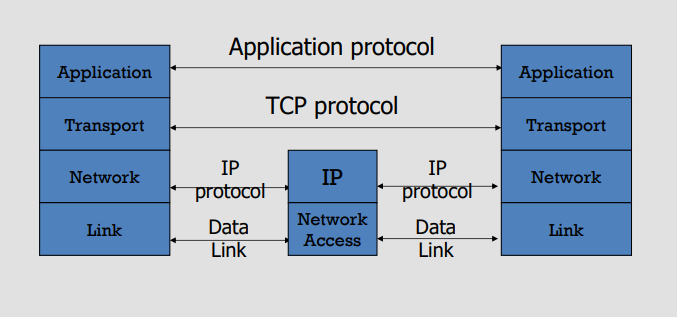
|
|
||||||
|
|
||||||
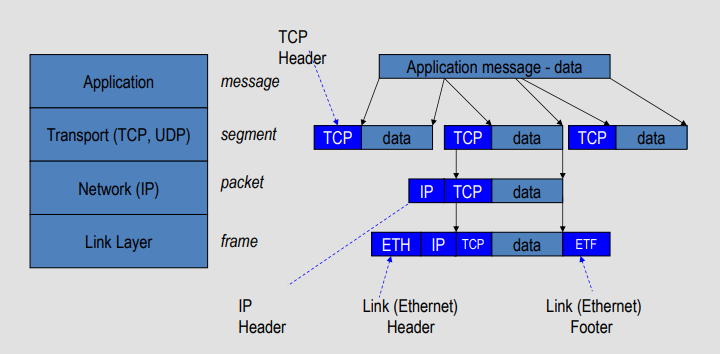
|
|
||||||
|
|
||||||
### Wireshark
|
|
||||||
|
|
||||||
Wireshark is a packet sniffer and protocol analyzer
|
|
||||||
|
|
||||||
- Captures and analyzes frames
|
|
||||||
- Supports plugins
|
|
||||||
|
|
||||||
Usually required to run with administrator privileges
|
|
||||||
|
|
||||||
Setting the network interface in promiscuous mode captures traffic across the entire LAN segment and not just frames addressed to the machine
|
|
||||||
|
|
||||||
### Examining the link layer
|
|
||||||
|
|
||||||
When a packet arrives at the destination subnet, MAC address is used to deliver the packet
|
|
||||||
|
|
||||||
#### ARP: Address Resolution Protocol
|
|
||||||
|
|
||||||
- Each IP node (Host, Router) on LAN has ARP table
|
|
||||||
- ARP Table: IP/MAC address mappings for some LAN nodes
|
|
||||||
`< IP address; MAC address; TTL>`
|
|
||||||
- TTL (Time To Live): time after which address mapping will be forgotten (typically 20 min)
|
|
||||||
|
|
||||||
#### Lack of Source Authentication - ARP Spoofing (ARP Poisoning)
|
|
||||||
|
|
||||||
Send fake or 'spoofed', ARP messages to an Ethernet LAN.
|
|
||||||
|
|
||||||
- To have other machines associate IP addresses with the attacker’s MAC
|
|
||||||
|
|
||||||
Legitimate use
|
|
||||||
|
|
||||||
- Implementing redundancy and fault tolerance
|
|
||||||
|
|
||||||
#### ARP Poisoning (Spoofing) Defense
|
|
||||||
|
|
||||||
Prevention
|
|
||||||
|
|
||||||
- Static ARP table
|
|
||||||
- DHCP Certification (use access control to ensure that hosts only use the IP addresses assigned to them, and that only authorized DHCP servers are accessible).
|
|
||||||
|
|
||||||
Detection
|
|
||||||
|
|
||||||
- Arpwatch (sending email when updates occur)
|
|
||||||
|
|
||||||
### Examining the network layer
|
|
||||||
|
|
||||||
Internet Protocol (IP)
|
|
||||||
|
|
||||||
Connectionless
|
|
||||||
|
|
||||||
- Unreliable
|
|
||||||
- Best effort
|
|
||||||
|
|
||||||
Notes:
|
|
||||||
|
|
||||||
- src and dest ports not parts of IP hdr
|
|
||||||
|
|
||||||
#### IP Protocol Functions (Summary)
|
|
||||||
|
|
||||||
Routing
|
|
||||||
|
|
||||||
- IP host knows location of router (gateway)
|
|
||||||
- IP gateway must know route to other networks
|
|
||||||
|
|
||||||
Fragmentation and reassembly
|
|
||||||
|
|
||||||
- If max-packet-size less than the user-data-size
|
|
||||||
|
|
||||||
Error reporting
|
|
||||||
|
|
||||||
- ICMP packet to source if packet is dropped
|
|
||||||
|
|
||||||
TTL field: decremented after every hop
|
|
||||||
|
|
||||||
- Packet dropped if TTL=0. Prevents infinite loops
|
|
||||||
|
|
||||||
#### Problem: no src IP authentication
|
|
||||||
|
|
||||||
Client is trusted to embed correct source IP
|
|
||||||
|
|
||||||
- Easy to override using raw sockets
|
|
||||||
|
|
||||||
- Libnet: a library for formatting raw packets with arbitrary IP headers
|
|
||||||
|
|
||||||
- Scapy: a python library for packet crafting
|
|
||||||
|
|
||||||
Anyone who owns their machine can send packets with arbitrary source IP
|
|
||||||
|
|
||||||
- ... response will be sent back to forged source IP
|
|
||||||
|
|
||||||
Implications:
|
|
||||||
|
|
||||||
- Anonymous DoS attacks;
|
|
||||||
- Anonymous infection attacks (e.g. slammer worm)
|
|
||||||
|
|
||||||
@@ -1,142 +0,0 @@
|
|||||||
# CSE4303 Introduction to Computer Security (Lecture 4)
|
|
||||||
|
|
||||||
## Network attacks
|
|
||||||
|
|
||||||
### Examining the transport layer
|
|
||||||
|
|
||||||
#### Transmission Control Protocol (TCP)
|
|
||||||
|
|
||||||
Connection-oriented, preserves order
|
|
||||||
|
|
||||||
- Sender
|
|
||||||
- Break data into packets
|
|
||||||
- Attach packet numbers
|
|
||||||
- Receiver
|
|
||||||
- Acknowledge receipt; lost packets are resent
|
|
||||||
- Reassemble packets in correct order
|
|
||||||
|
|
||||||
#### Security Problems
|
|
||||||
|
|
||||||
1. Network packets pass by untrusted hosts
|
|
||||||
- Eavesdropping, packet sniffing
|
|
||||||
- Especially easy when attacker controls a machine close to victim (e.g. WiFi routers)
|
|
||||||
2. TCP state easily obtained by eavesdropping
|
|
||||||
- Enables spoofing and session hijacking
|
|
||||||
3. Denial of Service (DoS) vulnerabilities
|
|
||||||
|
|
||||||
#### TCP SYN Flood I: low rate (DoS Bug)
|
|
||||||
|
|
||||||
Low rate SYN flood defenses
|
|
||||||
|
|
||||||
Correct Solution:
|
|
||||||
|
|
||||||
Syncookies: remove state from server
|
|
||||||
|
|
||||||
Small performance overhead
|
|
||||||
|
|
||||||
Hijacking Existing TCP connection
|
|
||||||
|
|
||||||
- A, B trusted connection
|
|
||||||
- Send packets with predictable seq numbers
|
|
||||||
|
|
||||||
- E impersonates B to A
|
|
||||||
- DoS B’s queue
|
|
||||||
- Sends packets to A that
|
|
||||||
resemble B’s transmission
|
|
||||||
- E cannot receive, but may
|
|
||||||
execute commands on A
|
|
||||||
|
|
||||||
## Routing Security
|
|
||||||
|
|
||||||
Routing Protocols
|
|
||||||
|
|
||||||
- ARP (addr resolution protocol): IP addr ⟶ eth addr
|
|
||||||
Security issues: (local network attacks)
|
|
||||||
- Node A can confuse gateway into sending it traffic for Node B
|
|
||||||
- By proxying traffic, node A can read/inject packets
|
|
||||||
into B’s session (e.g. WiFi networks)
|
|
||||||
- OSPF: used for routing within an AS
|
|
||||||
- BGP: routing between Autonomous Systems
|
|
||||||
Security issues: unauthenticated route updates
|
|
||||||
- Anyone can cause entire Internet to send traffic
|
|
||||||
for a victim IP to attacker’s address
|
|
||||||
- Example: Youtube-Pakistan mishap (see DDoS lecture)
|
|
||||||
- Anyone can hijack route to victim
|
|
||||||
|
|
||||||
### Security Issues
|
|
||||||
|
|
||||||
- BGP path attestations are un-authenticated
|
|
||||||
- Anyone can inject advertisements for arbitrary routes
|
|
||||||
- Advertisement will propagate everywhere
|
|
||||||
- Used for DoS, spam, and eavesdropping (details in DDoS lecture)
|
|
||||||
- Often a result of human error
|
|
||||||
|
|
||||||
Solutions:
|
|
||||||
|
|
||||||
- RPKI: AS obtains a certificate (ROA) from regional authority (RIR) and attaches ROA to path advertisement.
|
|
||||||
Advertisements without a valid ROA are ignored. Defends against a malicious AS
|
|
||||||
- SBGP: sign every hop of a path advertisement
|
|
||||||
|
|
||||||
### Domain Name System
|
|
||||||
|
|
||||||
DNS Root Name Servers
|
|
||||||
|
|
||||||
- Hierarchical service
|
|
||||||
- Root name servers for toplevel domains
|
|
||||||
- Authoritative name servers
|
|
||||||
for subdomains
|
|
||||||
- Local name resolvers contact
|
|
||||||
authoritative servers when
|
|
||||||
they do not know a name
|
|
||||||
|
|
||||||
#### DNS Lookup Example
|
|
||||||
|
|
||||||
#### Caching
|
|
||||||
|
|
||||||
- DNS responses are cached
|
|
||||||
- Quick response for repeated translations
|
|
||||||
- Note: NS records for domains also cached
|
|
||||||
- DNS negative queries are cached
|
|
||||||
- Save time for nonexistent sites, e.g. misspelling
|
|
||||||
- Cached data periodically times out
|
|
||||||
- Lifetime (TTL) of data controlled by owner of data
|
|
||||||
- TTL passed with every record
|
|
||||||
|
|
||||||
DNS Packet
|
|
||||||
|
|
||||||
- Query ID:
|
|
||||||
- 16 bit random value
|
|
||||||
- Links response to query
|
|
||||||
|
|
||||||
#### Basic DNS Vulnerabilities
|
|
||||||
|
|
||||||
- Users/hosts trust the host-address mapping
|
|
||||||
provided by DNS:
|
|
||||||
- Used as basis for many security policies:
|
|
||||||
Browser same origin policy, URL address bar
|
|
||||||
- Obvious problems
|
|
||||||
- Interception of requests or compromise of DNS servers can
|
|
||||||
result in incorrect or malicious responses
|
|
||||||
- e.g.: malicious access point in a Cafe
|
|
||||||
- Solution - authenticated requests/responses
|
|
||||||
- Provided by DNSsec … but few use DNSsec
|
|
||||||
|
|
||||||
### DNS cache poisoning (a la Kaminsky’08)
|
|
||||||
|
|
||||||

|
|
||||||
|
|
||||||
#### DNS poisoning attacks in the wild
|
|
||||||
|
|
||||||
- January 2005, the domain name for a large New York ISP, Panix, was hijacked to a site in Australia.
|
|
||||||
- In November 2004, Google and Amazon users were sent to Med Network Inc., an online pharmacy
|
|
||||||
- In March 2003, a group dubbed the "Freedom Cyber Force Militia" hijacked visitors to the Al-Jazeera Web site and presented them with the message "God Bless Our Troops"
|
|
||||||
|
|
||||||
### Summary
|
|
||||||
|
|
||||||
- Core protocols not designed for security
|
|
||||||
- Eavesdropping, Packet injection, Route stealing, DNS poisoning
|
|
||||||
- Patched over time to prevent basic attacks
|
|
||||||
- More secure variants exist :
|
|
||||||
- IP $\to$ IPsec
|
|
||||||
- DNS $\to$ DNSsec
|
|
||||||
- BGP $\to$ sBGPs
|
|
||||||
@@ -1,79 +0,0 @@
|
|||||||
# CSE4303 Introduction to Computer Security (Lecture 5)
|
|
||||||
|
|
||||||
## Cryptography: Foundations
|
|
||||||
|
|
||||||
### Definitions
|
|
||||||
|
|
||||||
Cryptography is the study of techniques that enable secure communication and computation in the presence of adversaries, by providing formal guarantees such as confidentiality, integrity, and authenticity.
|
|
||||||
|
|
||||||
Cryptanalysis is the study of techniques for breaking cryptographic systems, by recovering secret information or violating security guarantees without knowing the secret key
|
|
||||||
|
|
||||||
### Background: security guarantee
|
|
||||||
|
|
||||||
- Well-defined statement about difficulty of compromising a system
|
|
||||||
- ...with clear implicit or explicit assumptions about:
|
|
||||||
- Parameters of the system
|
|
||||||
- Threat model
|
|
||||||
- Attack surfaces
|
|
||||||
- Example: "A one-time pad cipher is secure against any cryptanalysis, including a brute-force attack, assuming:
|
|
||||||
- the key is the same length as the plaintext,
|
|
||||||
- the key is truly random, and
|
|
||||||
- the key is never re-used.
|
|
||||||
- Example: "Given that keys remain uncompromised (by human error, side channel, etc.), recovering an RSA private key from a given public key is at least as hard as integer factorization."
|
|
||||||
- I.e. we can reduce RSA to integer factorization.
|
|
||||||
- Note: correct implementation is not guaranteed!
|
|
||||||
- Non-example: "This app is secure."
|
|
||||||
- Empty claim: what does it mean?
|
|
||||||
|
|
||||||
### Overview: Encryption and Decryption
|
|
||||||
|
|
||||||
- The message m is called the plaintext.
|
|
||||||
- Alice will convert plaintext m to an encrypted form using an encryption algorithm E that outputs a ciphertext c for m
|
|
||||||
|
|
||||||
#### Cryptography goals
|
|
||||||
|
|
||||||
- Confidentiality:
|
|
||||||
- Mallory and Eve cannot recover original message from ciphertext
|
|
||||||
- Integrity:
|
|
||||||
- Mallory cannot modify message from Alice to Bob without detection
|
|
||||||
by Bob
|
|
||||||
- Authenticity:
|
|
||||||
- Mallory cannot craft a message that Bob would accept as coming from Alice
|
|
||||||
|
|
||||||
#### Cryptosystem compoents
|
|
||||||
|
|
||||||
1. The set of possible plaintexts (M)
|
|
||||||
2. The set of possible ciphertexts (C)
|
|
||||||
3. The set of encryption keys (K)
|
|
||||||
4. The set of decryption keys (usually K as well)
|
|
||||||
5. The correspondence between encryption keys and decryption
|
|
||||||
keys
|
|
||||||
6. The encryption algorithm to use (E)
|
|
||||||
7. The decryption algorithm to use (D)
|
|
||||||
|
|
||||||
#### Symmetric ciphers:
|
|
||||||
|
|
||||||
A cipher defined over $(K,M,C)$ is a pair of efficient algorithms $(E,D)$ where $E: K\times M\to C$ and $D: K\times C \to M$
|
|
||||||
|
|
||||||
Correctness Property:
|
|
||||||
|
|
||||||
$\forall m\in M, \exists k\in K$, $E(k,m) = c\in C$, and $D(k,c) = m$
|
|
||||||
|
|
||||||
- $D$ and $E$ are often efficient (polynomial time | concrete time)
|
|
||||||
- $E$ is encryption, often randomized.
|
|
||||||
- $D$ is decryption, always deterministic.
|
|
||||||
|
|
||||||
#### Threat models
|
|
||||||
|
|
||||||
Attackers may have:
|
|
||||||
|
|
||||||
- collection of ciphertexts (ciphertext-only attack)
|
|
||||||
- collection of plaintext/ciphertext pairs (known plaintext attack: KPA )
|
|
||||||
- collection of plaintext/ciphertext pairs for plaintexts selected by the attacker (chosen plaintext attack: CPA )
|
|
||||||
- collection of plaintext/ciphertext pairs for ciphertexts selected by the attacker (chosen ciphertext attack: CCA/CCA2 )
|
|
||||||
|
|
||||||
### Symmetric (shared-key) encryption
|
|
||||||
|
|
||||||
Refer to this lecture notes
|
|
||||||
|
|
||||||
[CSE442T Lecture 1](https://notenextra.trance-0.com/CSE442T/CSE442T_L1/)
|
|
||||||
@@ -1,5 +0,0 @@
|
|||||||
# CSE4303 Introduction to Computer Security (Lecture 6)
|
|
||||||
|
|
||||||
Refer to this lecture notes
|
|
||||||
|
|
||||||
[CSE442T Lecture 3](https://notenextra.trance-0.com/CSE442T/CSE442T_L3/)
|
|
||||||
@@ -1,144 +0,0 @@
|
|||||||
# CSE4303 Introduction to Computer Security (Lecture 7)
|
|
||||||
|
|
||||||
## Cryptography in Symmetric Systems
|
|
||||||
|
|
||||||
### Symmetric systems
|
|
||||||
|
|
||||||
Symmetric (shared-key) encryption
|
|
||||||
|
|
||||||
- Classical techniques
|
|
||||||
- Computer-aided techniques
|
|
||||||
- Formal reasoning
|
|
||||||
- Realizations:
|
|
||||||
- Stream ciphers
|
|
||||||
- Block ciphers
|
|
||||||
|
|
||||||
## Stream ciphers
|
|
||||||
|
|
||||||
1. Operate on PT one bit at a time (usually), as a bit "stream"
|
|
||||||
2. Generate arbitrarily long keystream on demand
|
|
||||||
|
|
||||||
### Keystream
|
|
||||||
|
|
||||||
Keystream $G(k)$ generated from key $k$.
|
|
||||||
|
|
||||||
Encryption:
|
|
||||||
$$
|
|
||||||
E(k,m) = m \oplus G(k)
|
|
||||||
$$
|
|
||||||
|
|
||||||
Decryption:
|
|
||||||
$$
|
|
||||||
D(k,c) = c \oplus G(k)
|
|
||||||
$$
|
|
||||||
|
|
||||||
### Security abstraction
|
|
||||||
|
|
||||||
1. XOR transfers randomness of keystream to randomness of CT regardless of PT’s content
|
|
||||||
2. Security depends on $G$ being "practically" indistinguishable from random string and "practically" unpredictable
|
|
||||||
3. Idea: shouldn’t be able to predict next bit of generator given all bits seen so far
|
|
||||||
|
|
||||||
### Keystream $G(k)$
|
|
||||||
|
|
||||||
- Idea: shouldn’t be able to predict next bit of generator given all bits seen so far
|
|
||||||
- Strategies and challenges: many!
|
|
||||||
|
|
||||||
#### Idea that doesn’t quite work: Linear Feedback Shift Register (LFSR)
|
|
||||||
|
|
||||||
- Choice of feedback: by algebra
|
|
||||||
- Pro: fast, statistically close to random
|
|
||||||
- Problem: susceptible to cryptanalysis (because linear)
|
|
||||||
|
|
||||||
#### LFSR-based modifications
|
|
||||||
|
|
||||||
- Use non-linear combo of multiple LFSRs
|
|
||||||
- Use controlled clocking (e.g. only cycle the LFSR when another LFSR outputs a 1)
|
|
||||||
- Etc.
|
|
||||||
|
|
||||||
#### Others
|
|
||||||
|
|
||||||
- Modular arithmetic-based constructions
|
|
||||||
- Other algebraic constructions
|
|
||||||
|
|
||||||
### Hazards
|
|
||||||
|
|
||||||
1. Weak PRG
|
|
||||||
2. Key re-use
|
|
||||||
3. Predictable effect of modifying CT on decrypted PT
|
|
||||||
|
|
||||||
#### Weak PRG
|
|
||||||
|
|
||||||
- Makes semantic security impossible
|
|
||||||
|
|
||||||
#### Key re-use
|
|
||||||
|
|
||||||
Suppose:
|
|
||||||
$$
|
|
||||||
c_1 = m_1 \oplus G(k)
|
|
||||||
$$
|
|
||||||
and
|
|
||||||
$$
|
|
||||||
c_2 = m_2 \oplus G(k)
|
|
||||||
$$
|
|
||||||
|
|
||||||
Then:
|
|
||||||
$$
|
|
||||||
c_1 \oplus c_2 = m_1 \oplus m_2
|
|
||||||
$$
|
|
||||||
|
|
||||||
This may be enough to recover $m_1$ or $m_2$ using natural language properties.
|
|
||||||
|
|
||||||
##### IV (Initialization Vector)
|
|
||||||
|
|
||||||
Used to avoid key re-use:
|
|
||||||
|
|
||||||
- IV incremented per frame
|
|
||||||
- But repeats after $2^{24}$ frames
|
|
||||||
- Sometimes resets to 0
|
|
||||||
- Enough to recover key within minutes
|
|
||||||
|
|
||||||
Note:
|
|
||||||
|
|
||||||
- Happens if keystream period is too short
|
|
||||||
- Real-world example: WEP attack (802.11b)
|
|
||||||
|
|
||||||
#### Predictable modification of ciphertext
|
|
||||||
|
|
||||||
If attacker modifies ciphertext by XORing $p$:
|
|
||||||
|
|
||||||
Ciphertext becomes:
|
|
||||||
$$
|
|
||||||
(m \oplus k) \oplus p
|
|
||||||
$$
|
|
||||||
|
|
||||||
Decryption yields:
|
|
||||||
$$
|
|
||||||
m \oplus p
|
|
||||||
$$
|
|
||||||
|
|
||||||
- Affects integrity
|
|
||||||
- Not CCA-secure for integrity
|
|
||||||
|
|
||||||
### Summary: Stream ciphers
|
|
||||||
|
|
||||||
Pros
|
|
||||||
|
|
||||||
- Fast
|
|
||||||
- Memory-efficient
|
|
||||||
- No minimum PT size
|
|
||||||
|
|
||||||
Cons
|
|
||||||
|
|
||||||
- Require good PRG
|
|
||||||
- Can never re-use key
|
|
||||||
- No integrity mechanism
|
|
||||||
|
|
||||||
Note
|
|
||||||
|
|
||||||
- Integrity mechanisms exist for other symmetric ciphers (block ciphers)
|
|
||||||
- "Authenticated encryption"
|
|
||||||
|
|
||||||
Examples / Uses
|
|
||||||
|
|
||||||
- RC4: legacy stream cipher (e.g. WEP)
|
|
||||||
- ChaCha / Salsa: Android cell phone encryption (Adiantum)
|
|
||||||
@@ -1,320 +0,0 @@
|
|||||||
# CSE4303 Introduction to Computer Security (Lecture 8)
|
|
||||||
|
|
||||||
## Block ciphers
|
|
||||||
|
|
||||||
1. Operate on PT one block at a time
|
|
||||||
2. Use same key for multiple blocks (with caveats)
|
|
||||||
3. Chaining modes intertwine successive blocks of CT (or not)
|
|
||||||
|
|
||||||
## Security abstraction
|
|
||||||
|
|
||||||
View cipher as a Pseudo-Random Permutation (PRP)
|
|
||||||
|
|
||||||
### Background: Pseudo-Random Function (PRF)
|
|
||||||
|
|
||||||
Defined over $(K,X,Y)$:
|
|
||||||
$$
|
|
||||||
F : K \times X \to Y
|
|
||||||
$$
|
|
||||||
|
|
||||||
Such that there exists an efficient algorithm to evaluate $F(k,x)$.
|
|
||||||
|
|
||||||
Let:
|
|
||||||
|
|
||||||
- $\text{Funs}[X,Y]$ = set of all functions from $X$ to $Y$
|
|
||||||
- $S_F = \{ F(k,\cdot) \mid k \in K \}$
|
|
||||||
|
|
||||||
Intuition:
|
|
||||||
|
|
||||||
A PRF is secure if a random function in $\text{Funs}[X,Y]$ is indistinguishable from a random function in $S_F$.
|
|
||||||
|
|
||||||
Adversarial game:
|
|
||||||
|
|
||||||
- Challenger samples $k \leftarrow K$
|
|
||||||
- Or samples $f \leftarrow \text{Funs}[X,Y]$
|
|
||||||
- Adversary queries oracle with $x \in X$
|
|
||||||
- Receives either $F(k,x)$ or $f(x)$
|
|
||||||
- Must distinguish
|
|
||||||
|
|
||||||
Goal: adversary’s advantage negligible
|
|
||||||
|
|
||||||
## PRP Definition
|
|
||||||
|
|
||||||
Defined over $(K,X)$:
|
|
||||||
$$
|
|
||||||
E : K \times X \to X
|
|
||||||
$$
|
|
||||||
|
|
||||||
Such that:
|
|
||||||
|
|
||||||
1. Efficient deterministic algorithm to evaluate $E(k,x)$
|
|
||||||
2. $E(k,\cdot)$ is one-to-one
|
|
||||||
3. Efficient inversion algorithm $D(k,y)$ exists
|
|
||||||
|
|
||||||
i.e., a PRF that is an invertible one-to-one mapping from message space to message space
|
|
||||||
|
|
||||||
## Secure PRP
|
|
||||||
|
|
||||||
Let $\text{Perms}[X]$ be all permutations on $X$.
|
|
||||||
|
|
||||||
Intuition:
|
|
||||||
|
|
||||||
A PRP is secure if a random permutation in $\text{Perms}[X]$ is indistinguishable from a random element of:
|
|
||||||
$$
|
|
||||||
S_E = \{ E(k,\cdot) \mid k \in K \}
|
|
||||||
$$
|
|
||||||
|
|
||||||
Adversarial game:
|
|
||||||
|
|
||||||
- Challenger samples $k \leftarrow K$
|
|
||||||
- Or $\pi \leftarrow \text{Perms}[X]$
|
|
||||||
- Adversary queries $x \in X$
|
|
||||||
- Receives either $E(k,x)$ or $\pi(x)$
|
|
||||||
- Must distinguish
|
|
||||||
|
|
||||||
Goal: negligible advantage
|
|
||||||
|
|
||||||
## Block cipher constructions
|
|
||||||
|
|
||||||
### Feistel network
|
|
||||||
|
|
||||||
Given:
|
|
||||||
$$
|
|
||||||
f_1, \dots, f_d : \{0,1\}^n \to \{0,1\}^n
|
|
||||||
$$
|
|
||||||
|
|
||||||
Build invertible function:
|
|
||||||
$$
|
|
||||||
F : \{0,1\}^{2n} \to \{0,1\}^{2n}
|
|
||||||
$$
|
|
||||||
|
|
||||||
Let input be split into $(L_0, R_0)$.
|
|
||||||
|
|
||||||
Round $i$:
|
|
||||||
$$
|
|
||||||
L_i = R_{i-1}
|
|
||||||
$$
|
|
||||||
$$
|
|
||||||
R_i = L_{i-1} \oplus f_i(R_{i-1})
|
|
||||||
$$
|
|
||||||
|
|
||||||
#### Invertibility
|
|
||||||
|
|
||||||
$$
|
|
||||||
R_{i-1} = L_i
|
|
||||||
$$
|
|
||||||
$$
|
|
||||||
L_{i-1} = R_i \oplus f_i(L_i)
|
|
||||||
$$
|
|
||||||
|
|
||||||
Thus Feistel is invertible regardless of whether $f_i$ is invertible.
|
|
||||||
|
|
||||||
### Luby–Rackoff Theorem (1985)
|
|
||||||
|
|
||||||
If $f$ is a secure PRF, then 3-round Feistel is a secure PRP.
|
|
||||||
|
|
||||||
### DES (Data Encryption Standard) — 1976
|
|
||||||
|
|
||||||
- 16-round Feistel network
|
|
||||||
- 64-bit block size
|
|
||||||
- 56-bit key
|
|
||||||
- Round functions:
|
|
||||||
$$
|
|
||||||
f_i(x) = F(k_i, x)
|
|
||||||
$$
|
|
||||||
|
|
||||||
Round function uses:
|
|
||||||
|
|
||||||
- S-box (substitution box) — non-linear
|
|
||||||
- P-box (permutation box)
|
|
||||||
|
|
||||||
To invert: use keys in reverse order.
|
|
||||||
|
|
||||||
Problem: 56-bit keyspace too small today (brute-force feasible).
|
|
||||||
|
|
||||||
### Substitution–Permutation Network (SPN)
|
|
||||||
|
|
||||||
Rounds of:
|
|
||||||
|
|
||||||
- Substitution (S-box layer)
|
|
||||||
- Permutation (P-layer)
|
|
||||||
- XOR with round key
|
|
||||||
|
|
||||||
All layers invertible.
|
|
||||||
|
|
||||||
### AES (Advanced Encryption Standard) — 2000
|
|
||||||
|
|
||||||
- 10 substitution-permutation rounds (128-bit key version)
|
|
||||||
- 128-bit block size
|
|
||||||
|
|
||||||
Each round includes:
|
|
||||||
|
|
||||||
- ByteSub (1-byte S-box)
|
|
||||||
- ShiftRows
|
|
||||||
- MixColumns
|
|
||||||
- AddRoundKey
|
|
||||||
|
|
||||||
Key sizes:
|
|
||||||
|
|
||||||
- 128-bit
|
|
||||||
- 192-bit
|
|
||||||
- 256-bit
|
|
||||||
|
|
||||||
Currently de facto standard symmetric-key cipher (e.g. TLS/SSL).
|
|
||||||
|
|
||||||
## Block cipher modes
|
|
||||||
|
|
||||||
### Challenge
|
|
||||||
|
|
||||||
Encrypt PTs longer than one block using same key while maintaining security.
|
|
||||||
|
|
||||||
### ECB (Electronic Codebook)
|
|
||||||
|
|
||||||
Encrypt blocks independently:
|
|
||||||
$$
|
|
||||||
c_i = E(k, m_i)
|
|
||||||
$$
|
|
||||||
|
|
||||||
Problem:
|
|
||||||
|
|
||||||
If $m_1 = m_2$, then:
|
|
||||||
$$
|
|
||||||
c_1 = c_2
|
|
||||||
$$
|
|
||||||
|
|
||||||
Not semantically secure.
|
|
||||||
|
|
||||||
#### Formal non-security argument
|
|
||||||
|
|
||||||
Two-block challenge:
|
|
||||||
|
|
||||||
- Adversary submits:
|
|
||||||
- $m_0 = \text{"Hello World"}$
|
|
||||||
- $m_1 = \text{"Hello Hello"}$
|
|
||||||
- If $c_1 = c_2$, output 0; else 1
|
|
||||||
|
|
||||||
Advantage = 1
|
|
||||||
|
|
||||||
### CPA model (Chosen Plaintext Attack)
|
|
||||||
|
|
||||||
Attacker:
|
|
||||||
|
|
||||||
- Sees many PT/CT pairs under same key
|
|
||||||
- Can submit arbitrary PTs
|
|
||||||
|
|
||||||
Definition:
|
|
||||||
$$
|
|
||||||
\text{Adv}_{CPA}[A,E] =
|
|
||||||
\left|
|
|
||||||
\Pr[\text{EXP}(0)=1] - \Pr[\text{EXP}(1)=1]
|
|
||||||
\right|
|
|
||||||
$$
|
|
||||||
|
|
||||||
Must be negligible.
|
|
||||||
|
|
||||||
ECB fails CPA security.
|
|
||||||
|
|
||||||
### Moral
|
|
||||||
|
|
||||||
If same secret key is used multiple times, given same PT twice, encryption must produce different CT outputs.
|
|
||||||
|
|
||||||
## Secure block modes
|
|
||||||
|
|
||||||
### Idea
|
|
||||||
|
|
||||||
Augment key with:
|
|
||||||
|
|
||||||
- Per-block nonce
|
|
||||||
- Or chaining data from prior blocks
|
|
||||||
|
|
||||||
### CBC (Cipher Block Chaining)
|
|
||||||
|
|
||||||
$$
|
|
||||||
c_1 = E(k, m_1 \oplus IV)
|
|
||||||
$$
|
|
||||||
$$
|
|
||||||
c_i = E(k, m_i \oplus c_{i-1})
|
|
||||||
$$
|
|
||||||
|
|
||||||
IV must be random/unpredictable.
|
|
||||||
|
|
||||||
### CFB (Cipher Feedback)
|
|
||||||
|
|
||||||
Uses previous ciphertext as input feedback into block cipher.
|
|
||||||
|
|
||||||
### OFB (Output Feedback)
|
|
||||||
|
|
||||||
$$
|
|
||||||
s_i = E(k, s_{i-1})
|
|
||||||
$$
|
|
||||||
$$
|
|
||||||
c_i = m_i \oplus s_i
|
|
||||||
$$
|
|
||||||
|
|
||||||
Can pre-compute keystream.
|
|
||||||
|
|
||||||
Acts like stream cipher.
|
|
||||||
|
|
||||||
### CTR (Counter Mode)
|
|
||||||
|
|
||||||
$$
|
|
||||||
c_i = m_i \oplus E(k, \text{nonce} \| \text{counter}_i)
|
|
||||||
$$
|
|
||||||
|
|
||||||
Encryption and decryption parallelizable.
|
|
||||||
|
|
||||||
Nonce must be unique.
|
|
||||||
|
|
||||||
### GCM (Galois Counter Mode)
|
|
||||||
|
|
||||||
- Most popular ("AES-GCM")
|
|
||||||
- Provides authenticated encryption
|
|
||||||
- Confidentiality + integrity
|
|
||||||
|
|
||||||
## Nonce-based semantic security
|
|
||||||
|
|
||||||
Encryption:
|
|
||||||
$$
|
|
||||||
c = E(k, m, n)
|
|
||||||
$$
|
|
||||||
|
|
||||||
Adversarial experiment:
|
|
||||||
|
|
||||||
- Challenger picks $k$
|
|
||||||
- Adversary submits $(m_{i,0}, m_{i,1})$ and nonce $n_i$
|
|
||||||
- Receives $c_i = E(k, m_{i,b}, n_i)$
|
|
||||||
- Nonces must be distinct
|
|
||||||
|
|
||||||
Definition:
|
|
||||||
$$
|
|
||||||
\text{Adv}_{nCPA}[A,E] =
|
|
||||||
\left|
|
|
||||||
\Pr[\text{EXP}(0)=1] - \Pr[\text{EXP}(1)=1]
|
|
||||||
\right|
|
|
||||||
$$
|
|
||||||
|
|
||||||
In practice:
|
|
||||||
|
|
||||||
- CBC: IV must be random
|
|
||||||
- CTR/GCM: nonce must be unique but not necessarily random
|
|
||||||
|
|
||||||
## Symmetric Encryption Summary
|
|
||||||
|
|
||||||
### Stream Ciphers
|
|
||||||
|
|
||||||
- Rely on secure PRG
|
|
||||||
- No key re-use
|
|
||||||
- Fast
|
|
||||||
- Low memory
|
|
||||||
- Less robust
|
|
||||||
- No built-in integrity
|
|
||||||
|
|
||||||
### Block Ciphers
|
|
||||||
|
|
||||||
- Rely on secure PRP
|
|
||||||
- Allow key re-use across blocks (secure mode required)
|
|
||||||
- Provide authenticated encryption in some modes (e.g. GCM)
|
|
||||||
- Slower
|
|
||||||
- Higher memory
|
|
||||||
- More robust
|
|
||||||
- Used in most practical secure systems (e.g. TLS)
|
|
||||||
@@ -1,254 +0,0 @@
|
|||||||
# CSE4303 Introduction to Computer Security (Lecture 9)
|
|
||||||
|
|
||||||
## Cryptographic Hash Functions
|
|
||||||
|
|
||||||
### What is a Hash Function
|
|
||||||
|
|
||||||
A hash function maps a variable-length input to a fixed-length output.
|
|
||||||
|
|
||||||
$h : X \to Y$
|
|
||||||
|
|
||||||
Typical examples:
|
|
||||||
- Java hashCode(): input is an Object, output is a 4-byte integer.
|
|
||||||
- String polynomial hash example:
|
|
||||||
$h("cs433s") = 'c' \cdot 31^6 + 's' \cdot 31^5 + \dots + 's'$
|
|
||||||
|
|
||||||
Key property:
|
|
||||||
- Domain $|X|$ is much larger than range $|Y|$.
|
|
||||||
- Collisions are unavoidable in principle since $|X| > |Y|$.
|
|
||||||
|
|
||||||
Main uses:
|
|
||||||
- Compact numerical representation
|
|
||||||
- Hash tables (Set, Map, dictionaries)
|
|
||||||
- Object comparison
|
|
||||||
- Integrity checking (fingerprint)
|
|
||||||
|
|
||||||
### Security Properties
|
|
||||||
|
|
||||||
Let $h : X \to Y$.
|
|
||||||
|
|
||||||
1. Preimage Resistance (One-way)
|
|
||||||
Given $y \in Y$, it is computationally infeasible to find $x \in X$ such that
|
|
||||||
$h(x) = y$.
|
|
||||||
|
|
||||||
2. Second Preimage Resistance (Weak collision resistance)
|
|
||||||
Given a specific $x \in X$, it is computationally infeasible to find $x' \neq x$ such that
|
|
||||||
$h(x') = h(x)$.
|
|
||||||
|
|
||||||
3. Collision Resistance (Strong collision resistance)
|
|
||||||
It is computationally infeasible to find any two distinct values $x, x' \in X$ such that
|
|
||||||
$h(x) = h(x')$.
|
|
||||||
|
|
||||||
Adversarial definition:
|
|
||||||
|
|
||||||
Let $H : M \to T$ where $|M|$ is much larger than $|T|$.
|
|
||||||
$H$ is collision resistant if for all efficient algorithms $A$:
|
|
||||||
|
|
||||||
$Adv_{CR}[A, H] = Pr[A$ outputs a collision for $H]$
|
|
||||||
|
|
||||||
is negligible.
|
|
||||||
|
|
||||||
### Generic Collision Attack (Birthday Attack)
|
|
||||||
|
|
||||||
Let $H : M \to \{0,1\}^n$.
|
|
||||||
|
|
||||||
Generic algorithm to find a collision in time on the order of $2^{n/2}$:
|
|
||||||
|
|
||||||
1. Choose $2^{n/2}$ random messages $m_1, \dots, m_{2^{n/2}}$.
|
|
||||||
2. Compute $t_i = H(m_i)$.
|
|
||||||
3. Look for $t_i = t_j$.
|
|
||||||
|
|
||||||
Birthday phenomenon:
|
|
||||||
|
|
||||||
If the output space size is $B$,
|
|
||||||
high collision probability greater than $50\%$ occurs with about $\sqrt{B}$ samples.
|
|
||||||
|
|
||||||
Thus:
|
|
||||||
- 128-bit hash gives about $2^{64}$ collision attack
|
|
||||||
- 256-bit hash gives about $2^{128}$ collision attack
|
|
||||||
|
|
||||||
### Practical Hash Functions
|
|
||||||
|
|
||||||
From performance and security table (AMD Opteron 2.2 GHz):
|
|
||||||
|
|
||||||
- MD5: 128 bits, completely broken since 2004
|
|
||||||
- SHA-1: 160 bits, practical collision attack demonstrated
|
|
||||||
- SHA-256: 256 bits
|
|
||||||
- SHA-512: 512 bits
|
|
||||||
- Whirlpool: 512 bits
|
|
||||||
|
|
||||||
SHA-1 collision example: SHAttered attack (Google and CWI).
|
|
||||||
Two different PDF files were produced with identical SHA-1 hash.
|
|
||||||
|
|
||||||
## Construction of Cryptographic Hash Functions
|
|
||||||
|
|
||||||
### Merkle-Damgard Construction
|
|
||||||
|
|
||||||
Given compression function:
|
|
||||||
|
|
||||||
$h : T \times X \to T$
|
|
||||||
|
|
||||||
We build:
|
|
||||||
|
|
||||||
$H : X^{\le L} \to T$
|
|
||||||
|
|
||||||
Process:
|
|
||||||
- Split message into blocks $m[0], m[1], \dots, m[L]$.
|
|
||||||
- Use fixed initialization vector $IV$.
|
|
||||||
- Iterate chaining:
|
|
||||||
|
|
||||||
$H_0 = IV$
|
|
||||||
$H_1 = h(H_0, m[0])$
|
|
||||||
$H_2 = h(H_1, m[1])$
|
|
||||||
$\dots$
|
|
||||||
$H_L = h(H_{L-1}, m[L])$
|
|
||||||
|
|
||||||
- Apply padding:
|
|
||||||
append $1000\ldots0$ concatenated with message length (64 bits).
|
|
||||||
If no space remains, add another block.
|
|
||||||
|
|
||||||
Theorem:
|
|
||||||
If compression function $h$ is collision resistant,
|
|
||||||
then $H$ is collision resistant.
|
|
||||||
|
|
||||||
### Davies-Meyer Compression from Block Cipher
|
|
||||||
|
|
||||||
Given block cipher:
|
|
||||||
|
|
||||||
$E : K \times \{0,1\}^n \to \{0,1\}^n$
|
|
||||||
|
|
||||||
Define compression function:
|
|
||||||
|
|
||||||
$h(H, m) = E(m, H) \oplus H$
|
|
||||||
|
|
||||||
If $E$ behaves like an ideal cipher,
|
|
||||||
finding a collision in $h$ takes about $2^{n/2}$ evaluations.
|
|
||||||
|
|
||||||
This is optimal for $n$-bit output.
|
|
||||||
|
|
||||||
### Example: SHA-256
|
|
||||||
|
|
||||||
Built using:
|
|
||||||
- Merkle-Damgard construction
|
|
||||||
- Davies-Meyer style compression
|
|
||||||
- Block cipher-like core: SHACAL-2
|
|
||||||
|
|
||||||
Structure:
|
|
||||||
- 512-bit message block
|
|
||||||
- 256-bit chaining value
|
|
||||||
- 256-bit output
|
|
||||||
|
|
||||||
## Applications for Integrity and Authentication
|
|
||||||
|
|
||||||
### Standalone Usage: Message Integrity
|
|
||||||
|
|
||||||
#### Application 1: Delayed Knowledge Verification
|
|
||||||
|
|
||||||
Idea:
|
|
||||||
Publish $h(secret)$ first.
|
|
||||||
Later reveal secret.
|
|
||||||
Anyone can recompute hash and verify.
|
|
||||||
|
|
||||||
Justification:
|
|
||||||
Preimage resistance ensures secret is hidden until revealed.
|
|
||||||
|
|
||||||
Example:
|
|
||||||
Stock market prediction commitment.
|
|
||||||
|
|
||||||
<details>
|
|
||||||
<summary>Example for delayed knowledge verification</summary>
|
|
||||||
|
|
||||||
1. Publish $H("Stock will rise on May 1")$.
|
|
||||||
2. On May 1, reveal the prediction string.
|
|
||||||
3. Anyone computes hash and checks equality.
|
|
||||||
|
|
||||||
</details>
|
|
||||||
|
|
||||||
#### Application 2: Password Storage
|
|
||||||
|
|
||||||
Model:
|
|
||||||
System must verify password but not store plaintext.
|
|
||||||
|
|
||||||
Solution:
|
|
||||||
Store hash of password.
|
|
||||||
During login:
|
|
||||||
- Hash input
|
|
||||||
- Compare with stored value
|
|
||||||
|
|
||||||
Example:
|
|
||||||
Linux stores hashed passwords in the /etc/shadow file.
|
|
||||||
Includes:
|
|
||||||
- Salt
|
|
||||||
- Password hash
|
|
||||||
- Metadata
|
|
||||||
|
|
||||||
Security relies on:
|
|
||||||
- One-way property
|
|
||||||
- Salting to prevent precomputed attacks
|
|
||||||
|
|
||||||
#### Application 3: Trusted Timestamping and Blockchains
|
|
||||||
|
|
||||||
Goal:
|
|
||||||
Prove document existed before a given date.
|
|
||||||
|
|
||||||
Methods:
|
|
||||||
- Publish document hash in newspaper.
|
|
||||||
- Time Stamping Authority signs hash.
|
|
||||||
- Publish hash in blockchain block.
|
|
||||||
|
|
||||||
Blockchain relies on:
|
|
||||||
- One-way hash functions
|
|
||||||
- Linking blocks via hash pointers
|
|
||||||
|
|
||||||
#### Application 4: Software Integrity with Secure Read-Only Space
|
|
||||||
|
|
||||||
Context:
|
|
||||||
Trusted read-only public space (for example official website).
|
|
||||||
|
|
||||||
Process:
|
|
||||||
1. Publisher computes $H(F_1), H(F_2), \dots, H(F_n)$.
|
|
||||||
2. Publish hashes publicly.
|
|
||||||
3. User downloads file $F_i$ and verifies hash.
|
|
||||||
|
|
||||||
If $H$ is collision resistant:
|
|
||||||
Attacker cannot modify file without detection.
|
|
||||||
|
|
||||||
No encryption required.
|
|
||||||
Public verifiability works if read-only space is trusted.
|
|
||||||
|
|
||||||
## Symmetric Crypto Authentication: MACs and AE
|
|
||||||
|
|
||||||
This section can also be found here [CSE442T Introduction to Cryptography (Lecture 18)](https://notenextra.trance-0.com/CSE442T/CSE442T_L18/#chapter-5-authentication)
|
|
||||||
|
|
||||||
### Message Authentication Codes (MACs)
|
|
||||||
|
|
||||||
Definition:
|
|
||||||
MAC $I = (S, V)$ over $(K, M, T)$
|
|
||||||
|
|
||||||
- $S(k, m) \to t$
|
|
||||||
- $V(k, m, t) \to$ yes or no
|
|
||||||
|
|
||||||
Security model:
|
|
||||||
Attacker can query $S(k, m_i)$.
|
|
||||||
Goal: produce new $(m, t)$ not previously seen such that $V$ accepts.
|
|
||||||
|
|
||||||
$Adv_{MAC}[A, I]$ must be negligible.
|
|
||||||
|
|
||||||
### MAC from PRF
|
|
||||||
|
|
||||||
Given PRF:
|
|
||||||
|
|
||||||
$F : K \times X \to Y$
|
|
||||||
|
|
||||||
Define MAC:
|
|
||||||
|
|
||||||
$S(k, m) = F(k, m)$
|
|
||||||
$V(k, m, t)$ accepts if $t = F(k, m)$
|
|
||||||
|
|
||||||
Theorem:
|
|
||||||
If $F$ is secure PRF and $|Y|$ is large,
|
|
||||||
then derived MAC is secure.
|
|
||||||
|
|
||||||
Condition:
|
|
||||||
$1 / |Y|$ must be negligible.
|
|
||||||
Example: $|Y| = 2^{80}$.
|
|
||||||
@@ -1,24 +0,0 @@
|
|||||||
export default {
|
|
||||||
index: "Course Description",
|
|
||||||
"---":{
|
|
||||||
type: 'separator'
|
|
||||||
},
|
|
||||||
CSE4303_E1: "Exam review",
|
|
||||||
CSE4303_L1: "Introduction to Computer Security (Lecture 1)",
|
|
||||||
CSE4303_L2: "Introduction to Computer Security (Lecture 2)",
|
|
||||||
CSE4303_L3: "Introduction to Computer Security (Lecture 3)",
|
|
||||||
CSE4303_L4: "Introduction to Computer Security (Lecture 4)",
|
|
||||||
CSE4303_L5: "Introduction to Computer Security (Lecture 5)",
|
|
||||||
CSE4303_L6: "Introduction to Computer Security (Lecture 6)",
|
|
||||||
CSE4303_L7: "Introduction to Computer Security (Lecture 7)",
|
|
||||||
CSE4303_L8: "Introduction to Computer Security (Lecture 8)",
|
|
||||||
CSE4303_L9: "Introduction to Computer Security (Lecture 9)",
|
|
||||||
CSE4303_L9: "Introduction to Computer Security (Lecture 9)",
|
|
||||||
CSE4303_L10: "Introduction to Computer Security (Lecture 10)",
|
|
||||||
CSE4303_L11: "Introduction to Computer Security (Lecture 11)",
|
|
||||||
CSE4303_L12: "Introduction to Computer Security (Lecture 12)",
|
|
||||||
CSE4303_L13: "Introduction to Computer Security (Lecture 13)",
|
|
||||||
CSE4303_L14: "Introduction to Computer Security (Lecture 14)",
|
|
||||||
CSE4303_L15: "Introduction to Computer Security (Lecture 15)",
|
|
||||||
CSE4303_L16: "Introduction to Computer Security (Lecture 16)"
|
|
||||||
}
|
|
||||||
@@ -1,133 +0,0 @@
|
|||||||
# CSE 4303 Introduction to Computer Security
|
|
||||||
|
|
||||||
**Term:** Spring 2026
|
|
||||||
**Credit awarded:** 3.0
|
|
||||||
**Course mode:** in-person
|
|
||||||
|
|
||||||
## Description and Pre-requisites
|
|
||||||
|
|
||||||
Secure computing requires the secure design, implementation, and use of systems and algorithms across many areas of computer science. Fundamentals of secure computing such as trust models and cryptography will lay the groundwork for studying key topics in the security of systems, networking, web design, machine learning algorithms, mobile applications, and physical devices. Human factors, privacy, and the law will also be considered. Hands-on practice exploring vulnerabilities and defenses using Linux, C, and Python in studios and lab assignments is a key component of the course.
|
|
||||||
|
|
||||||
**Prerequisites:** CSE 247 and either CSE 361 or CSE 332.
|
|
||||||
|
|
||||||
## Learning Objectives
|
|
||||||
|
|
||||||
1. Understand principles of security analysis
|
|
||||||
2. Explain key security concepts such as confidentiality
|
|
||||||
3. Explain the root causes of current security problems
|
|
||||||
4. Produce clear and concise descriptions of security problems on real world systems
|
|
||||||
5. Analyze systems for potential vulnerabilities
|
|
||||||
6. Gain hands-on experience using security tools to attack and defend vulnerable systems
|
|
||||||
|
|
||||||
## Meeting Time and Location
|
|
||||||
|
|
||||||
Tuesdays and Thursdays, 11:30 AM - 12:50 PM
|
|
||||||
Urbauer 218
|
|
||||||
|
|
||||||
## Instructor
|
|
||||||
|
|
||||||
**Jon Shidal**
|
|
||||||
shidalj@wustl.edu
|
|
||||||
Lopata 204A
|
|
||||||
|
|
||||||
**Office hours:** See Piazza pinned post.
|
|
||||||
|
|
||||||
## Textbook
|
|
||||||
|
|
||||||
**Strongly Recommended:** Wenliang Du, *Computer & Internet Security: A Hands-on Approach* (3rd ed.)
|
|
||||||
|
|
||||||
This book is the companion to the SEED labs from Kevin Du at Syracuse that we will use for many of our hands-on exercises.
|
|
||||||
|
|
||||||
- [Textbook website](https://www.handsonsecurity.net) with a few sample chapters and links to slides and Udemy videos
|
|
||||||
|
|
||||||
## Technologies
|
|
||||||
|
|
||||||
Laptop capable of running VM hypervisor (VirtualBox, or VMWare Fusion for Apple machines with an M1 or later processor chip)
|
|
||||||
|
|
||||||
## Educational Resources Used
|
|
||||||
|
|
||||||
- Canvas (main portal for class)
|
|
||||||
- Gradescope (assignment turnins)
|
|
||||||
- Piazza (course communication)
|
|
||||||
|
|
||||||
## Class Workflow, Assignment Types, and Grading
|
|
||||||
|
|
||||||
This class consists of lecture as well as a large hands-on studio component. A typical week (but not every week...) will consist of:
|
|
||||||
|
|
||||||
- **Pre-lecture prep work:** Materials to read or watch outside of class and prior to class/lecture
|
|
||||||
- **Lecture (typically on Tuesday):** in-class lecture over a new topic
|
|
||||||
- **Studio (typically on Thursday):** in-class hands-on group exercises. Graded on best effort and completion. Studios must be completed outside of class if they are not finished during the assigned class period.
|
|
||||||
|
|
||||||
There will also be additional homework assignments that should be completed individually outside of class.
|
|
||||||
|
|
||||||
### Other Assignment Types
|
|
||||||
|
|
||||||
- **Homeworks:** To be completed individually outside of class, graded on correctness
|
|
||||||
- **Midterm exam:** The midterm will be held in class on March 5th. It will cover all material up until that point in the semester
|
|
||||||
- **Final project:** The project will give you and your group mates an opportunity to take a deep dive into a particular security concept of your choice.
|
|
||||||
- **News reports:** Short summaries of security-related current events from credible news sources. You are required to complete 1. You may complete a second for extra credit.
|
|
||||||
|
|
||||||
### Grading Breakdown
|
|
||||||
|
|
||||||
| Assignment Type | Final Grade Percentage |
|
|
||||||
|----------------|------------------------|
|
|
||||||
| Studios | 28% |
|
|
||||||
| **Homeworks (total):** | **20%** |
|
|
||||||
| - HW 0 | 6% |
|
|
||||||
| - HW 1 | 5% |
|
|
||||||
| - HW 2 | 3% |
|
|
||||||
| - HW 3 | 3% |
|
|
||||||
| - HW 4 | 3% |
|
|
||||||
| Midterm Exam | 25% |
|
|
||||||
| Final Project | 25% |
|
|
||||||
| Course Evaluation | 1% |
|
|
||||||
| News Reports | 1% + 1% extra credit |
|
|
||||||
| **Total:** | **101%** |
|
|
||||||
|
|
||||||
A typical 10 point grading scale will be applied when converting number grades to letter grades: A (90+), B (80-89), C (70-79), D (60-69), F (<60). I will modify letter grades with +/- within 2 points of a boundary. I will not do any rounding of grades.
|
|
||||||
|
|
||||||
**Example:**
|
|
||||||
- 98.00: A+
|
|
||||||
- 97.99: A
|
|
||||||
- 92.0: A
|
|
||||||
- 91.99: A-
|
|
||||||
- 90.00: A-
|
|
||||||
- 89.99: B+
|
|
||||||
|
|
||||||
A grade of C- is required to receive a passing grade in this course if the course is being taken pass/fail.
|
|
||||||
|
|
||||||
## Course Policies
|
|
||||||
|
|
||||||
### Late Work/Extension Policy
|
|
||||||
|
|
||||||
Studio and Homework deadlines are organized in a way that you should be able to complete all assignments on-time. However, we understand things come up that require flexibility. To account for this, each student will be automatically given two "late coupons". A late coupon allows you to turn any Studio or Homework assignment in up to three days late without a grade penalty. You must notify the instructor via email prior to the assignment deadline to use a late coupon. Once you have used all late coupons, any late work will result in a 0. Late coupons may not be used on the exam, the final project, or news reports. Due to this built-in flexibility, no other extensions will normally be considered. Please contact the instructor ASAP to request an excused absence or special accommodation on any assignment if absolutely necessary.
|
|
||||||
|
|
||||||
### Regrade Requests
|
|
||||||
|
|
||||||
Effort will be made to grade work consistently across all students. If you believe your work was graded incorrectly, you may submit a regrade request via Gradescope explaining what you think was graded incorrectly (e.g. "Some of my work was on a different page and does not appear to have been seen by the grader.") within one week of grades being returned. Please note that questions about why an answer is incorrect are not regrade requests, and should be asked on Piazza for the benefit of everyone rather than submitted as regrade requests. If you are not sure whether your answer is correct, please ask on Piazza first.
|
|
||||||
|
|
||||||
### Collaboration
|
|
||||||
|
|
||||||
**Studios, lecture, Piazza, final project:** You are encouraged to work together with other students in groups of 2-3 for studios and the final project, and to fully embrace the public spaces of the class (class discussions on news and the topics of the days, Piazza) to maximize our chance to learn together. The benefit of learning in a class rather than individually is the chance to all engage the material together!
|
|
||||||
|
|
||||||
**Homeworks, news reports, and the exam** are to be completed individually to allow you to demonstrate your learning.
|
|
||||||
|
|
||||||
### Academic Integrity
|
|
||||||
|
|
||||||
Please refer to the [McKelvey Academic Integrity Policy](https://engineering.wustl.edu/academics/undergraduate-programs/undergraduate-academic-policies/academic-integrity.html).
|
|
||||||
|
|
||||||
From the University: In all academic work, the ideas and contributions of others (including generative artificial intelligence) must be appropriately acknowledged and work that is presented as original must be, in fact, original. You should familiarize yourself with the appropriate academic integrity policies of your academic program(s).
|
|
||||||
|
|
||||||
#### Note on AI Tools
|
|
||||||
|
|
||||||
Using an AI-content generator (such as OpenAI's ChatGPT or GitHub Copilot) to complete coursework without proper attribution or authorization is a form of academic dishonesty. Here are my rules for this course:
|
|
||||||
|
|
||||||
1. You may not ask generative AI to solve your homework for you. You may use generative AI as a tool to help you develop your own solution.
|
|
||||||
2. If your solution has bugs, you may use generative AI to help you find and understand the bugs so that you can fix them. You may not ask generative AI to fix the bugs for you.
|
|
||||||
3. If you use generative AI in one of the above legal ways, you should describe your conversation and what you learned. Please also list which generative AI model or tool was used.
|
|
||||||
|
|
||||||
### Ethics
|
|
||||||
|
|
||||||
In a computer security course, it is necessary to study many vulnerabilities and exploits. You will be acquiring theoretical and technical knowledge that could be used for good or for ill, and it is your responsibility as an ethical computer scientist to use it for good.
|
|
||||||
|
|
||||||
Our school is generous in providing us resources with which to learn and trusting us to use our knowledge wisely, and we as your instructors are trusting you with the same. Any attempt to use knowledge gained in this class, now or in the future, to compromise, gain unauthorized access to, or otherwise maliciously affect any university- or non-university-managed resource will be prosecuted to the full extent of all applicable Washington University polices and all local, state, and federal laws. Any such attempt will also earn the ire of your instructors and bring you dishonor and discredit as a scientist. Many legitimate means of practicing offensive and defensive techniques are available; there is no need to resort to illegitimate ones. If you have a question about whether testing a particular technique in a particular context beyond the scope of course assignments is permissible, please ask first.
|
|
||||||
@@ -1,31 +1,61 @@
|
|||||||
export default {
|
export default {
|
||||||
index: "Course Description",
|
menu: {
|
||||||
"---":{
|
title: 'Home',
|
||||||
type: 'separator'
|
type: 'menu',
|
||||||
|
items: {
|
||||||
|
index: {
|
||||||
|
title: 'Home',
|
||||||
|
href: '/'
|
||||||
|
},
|
||||||
|
about: {
|
||||||
|
title: 'About',
|
||||||
|
href: '/about'
|
||||||
|
},
|
||||||
|
contact: {
|
||||||
|
title: 'Contact Me',
|
||||||
|
href: '/contact'
|
||||||
|
}
|
||||||
|
},
|
||||||
},
|
},
|
||||||
Exam_reviews: "Exam reviews",
|
Math3200'CSE442T_link\s*:\s*(\{\s+.+\s+.+)\s+.+\s+.+\s+.+\s+(\},)'
|
||||||
CSE442T_L1: "Introduction to Cryptography (Lecture 1)",
|
Math429'CSE442T_link\s*:\s*(\{\s+.+\s+.+)\s+.+\s+.+\s+.+\s+(\},)'
|
||||||
CSE442T_L2: "Introduction to Cryptography (Lecture 2)",
|
Math4111'CSE442T_link\s*:\s*(\{\s+.+\s+.+)\s+.+\s+.+\s+.+\s+(\},)'
|
||||||
CSE442T_L3: "Introduction to Cryptography (Lecture 3)",
|
Math4121'CSE442T_link\s*:\s*(\{\s+.+\s+.+)\s+.+\s+.+\s+.+\s+(\},)'
|
||||||
CSE442T_L4: "Introduction to Cryptography (Lecture 4)",
|
Math4201'CSE442T_link\s*:\s*(\{\s+.+\s+.+)\s+.+\s+.+\s+.+\s+(\},)'
|
||||||
CSE442T_L5: "Introduction to Cryptography (Lecture 5)",
|
Math416'CSE442T_link\s*:\s*(\{\s+.+\s+.+)\s+.+\s+.+\s+.+\s+(\},)'
|
||||||
CSE442T_L6: "Introduction to Cryptography (Lecture 6)",
|
Math401'CSE442T_link\s*:\s*(\{\s+.+\s+.+)\s+.+\s+.+\s+.+\s+(\},)'
|
||||||
CSE442T_L7: "Introduction to Cryptography (Lecture 7)",
|
CSE332S'CSE442T_link\s*:\s*(\{\s+.+\s+.+)\s+.+\s+.+\s+.+\s+(\},)'
|
||||||
CSE442T_L8: "Introduction to Cryptography (Lecture 8)",
|
CSE347'CSE442T_link\s*:\s*(\{\s+.+\s+.+)\s+.+\s+.+\s+.+\s+(\},)'
|
||||||
CSE442T_L9: "Introduction to Cryptography (Lecture 9)",
|
CSE442T'CSE442T_link\s*:\s*(\{\s+.+\s+.+)\s+.+\s+.+\s+.+\s+(\},)'
|
||||||
CSE442T_L10: "Introduction to Cryptography (Lecture 10)",
|
CSE5313'CSE442T_link\s*:\s*(\{\s+.+\s+.+)\s+.+\s+.+\s+.+\s+(\},)'
|
||||||
CSE442T_L11: "Introduction to Cryptography (Lecture 11)",
|
CSE510'CSE442T_link\s*:\s*(\{\s+.+\s+.+)\s+.+\s+.+\s+.+\s+(\},)'
|
||||||
CSE442T_L12: "Introduction to Cryptography (Lecture 12)",
|
CSE559A'CSE442T_link\s*:\s*(\{\s+.+\s+.+)\s+.+\s+.+\s+.+\s+(\},)'
|
||||||
CSE442T_L13: "Introduction to Cryptography (Lecture 13)",
|
CSE5519'CSE442T_link\s*:\s*(\{\s+.+\s+.+)\s+.+\s+.+\s+.+\s+(\},)'
|
||||||
CSE442T_L14: "Introduction to Cryptography (Lecture 14)",
|
Swap: {
|
||||||
CSE442T_L15: "Introduction to Cryptography (Lecture 15)",
|
display: 'hidden',
|
||||||
CSE442T_L16: "Introduction to Cryptography (Lecture 16)",
|
theme:{
|
||||||
CSE442T_L17: "Introduction to Cryptography (Lecture 17)",
|
timestamp: true,
|
||||||
CSE442T_L18: "Introduction to Cryptography (Lecture 18)",
|
}
|
||||||
CSE442T_L19: "Introduction to Cryptography (Lecture 19)",
|
},
|
||||||
CSE442T_L20: "Introduction to Cryptography (Lecture 20)",
|
index: {
|
||||||
CSE442T_L21: "Introduction to Cryptography (Lecture 21)",
|
display: 'hidden',
|
||||||
CSE442T_L22: "Introduction to Cryptography (Lecture 22)",
|
theme:{
|
||||||
CSE442T_L23: "Introduction to Cryptography (Lecture 23)",
|
sidebar: false,
|
||||||
CSE442T_L24: "Introduction to Cryptography (Lecture 24)"
|
timestamp: true,
|
||||||
}
|
}
|
||||||
|
},
|
||||||
|
about: {
|
||||||
|
display: 'hidden',
|
||||||
|
theme:{
|
||||||
|
sidebar: false,
|
||||||
|
timestamp: true,
|
||||||
|
}
|
||||||
|
},
|
||||||
|
contact: {
|
||||||
|
display: 'hidden',
|
||||||
|
theme:{
|
||||||
|
sidebar: false,
|
||||||
|
timestamp: true,
|
||||||
|
}
|
||||||
|
}
|
||||||
|
}
|
||||||
@@ -85,7 +85,7 @@ TRPO = NPG + Linesearch + monotonic improvement theorem
|
|||||||
Pros
|
Pros
|
||||||
|
|
||||||
- Proper learning step
|
- Proper learning step
|
||||||
- [Monotonic improvement guarantee](../CSE510_L13.md#Monotonic-Improvement-Theorem)
|
- [Monotonic improvement guarantee](./CSE510_L13.md#Monotonic-Improvement-Theorem)
|
||||||
|
|
||||||
Cons
|
Cons
|
||||||
|
|
||||||
|
|||||||
@@ -90,6 +90,8 @@ Parameter explanations:
|
|||||||
|
|
||||||
IGM makes decentralized execution optimal with respect to the learned factorized value.
|
IGM makes decentralized execution optimal with respect to the learned factorized value.
|
||||||
|
|
||||||
|
## Linear Value Factorization
|
||||||
|
|
||||||
### VDN (Value Decomposition Networks)
|
### VDN (Value Decomposition Networks)
|
||||||
|
|
||||||
VDN assumes:
|
VDN assumes:
|
||||||
|
|||||||
@@ -1,101 +0,0 @@
|
|||||||
# CSE510 Deep Reinforcement Learning (Lecture 25)
|
|
||||||
|
|
||||||
> Restore human intelligence
|
|
||||||
|
|
||||||
## Linear Value Factorization
|
|
||||||
|
|
||||||
[link to paper](https://arxiv.org/abs/2006.00587)
|
|
||||||
|
|
||||||
### Why Linear Factorization works?
|
|
||||||
|
|
||||||
- Multi-agent reinforcement learning are mostly emprical
|
|
||||||
- Theoretical Model: Factored Multi-Agent Fitted Q-Iteration (FMA-FQI)
|
|
||||||
|
|
||||||
#### Theorem 1
|
|
||||||
|
|
||||||
It realize **Counterfactual** credit assignment mechanism.
|
|
||||||
|
|
||||||
Agent $i$:
|
|
||||||
|
|
||||||
$$
|
|
||||||
Q_i^{(t+1)}(s,a_i)=\mathbb{E}_{a_{-i}'}\left[y^{(t)}(s,a_i\oplus a_{-i}')\right]-\frac{n-1}{n}\mathbb{E}_{a'}\left[y^{(t)}(s,a')\right]
|
|
||||||
$$
|
|
||||||
|
|
||||||
Here $\mathbb{E}_{a_{-i}'}\left[y^{(t)}(s,a_i\oplus a_{-i}')\right]$ is the evaluation of $a_i$.
|
|
||||||
|
|
||||||
and $\mathbb{E}_{a'}\left[y^{(t)}(s,a')\right]$ is the baseline
|
|
||||||
|
|
||||||
The target $Q$-value: $y^{(t)}(s,a)=r+\gamma\max_{a'}Q_{tot}^{(t)}(s',a')$
|
|
||||||
|
|
||||||
#### Theorem 2
|
|
||||||
|
|
||||||
it has local convergence with on-policy training
|
|
||||||
|
|
||||||
##### Limitations of Linear Factorization
|
|
||||||
|
|
||||||
Linear: $Q_{tot}(s,a)=\sum_{i=1}^{n}Q_{i}(s,a_i)$
|
|
||||||
|
|
||||||
Limited Representation: Suboptimal (Prisoner's Dilemma)
|
|
||||||
|
|
||||||
|a_2\a_2| Action 1 | Action 2 |
|
|
||||||
|---|---|---|
|
|
||||||
|Action 1| **8** | -12 |
|
|
||||||
|Action 2| -12 | 0 |
|
|
||||||
|
|
||||||
After linear factorization:
|
|
||||||
|
|
||||||
|a_2\a_2| Action 1 | Action 2 |
|
|
||||||
|---|---|---|
|
|
||||||
|Action 1| -6.5 | -5 |
|
|
||||||
|Action 2| -5 | **-3.5** |
|
|
||||||
|
|
||||||
#### Theorem 3
|
|
||||||
|
|
||||||
it may diverge with off-policy training
|
|
||||||
|
|
||||||
### Perfect Alignment: IGM Factorization
|
|
||||||
|
|
||||||
- Individual-Global Maximization (IGM) Constraint
|
|
||||||
|
|
||||||
$$
|
|
||||||
\argmax_{a}Q_{tot}(s,a)=(\argmax_{a_1}Q_1(s,a_1), \dots, \argmax_{a_n}Q_n(s,a_n))
|
|
||||||
$$
|
|
||||||
|
|
||||||
- IGM Factorization: $Q_{tot} (s,a)=f(Q_1(s,a_1), \dots, Q_n(s,a_n))$
|
|
||||||
- Factorization function $f$ realizes all functions satsisfying IGM.
|
|
||||||
|
|
||||||
- FQI-IGM: Fitted Q-Iteration with IGM Factorization
|
|
||||||
|
|
||||||
#### Theorem 4
|
|
||||||
|
|
||||||
Convergence & optimality. FQI-IGM globally converges to the optimal value function in multi-agent MDPs.
|
|
||||||
|
|
||||||
### QPLEX: Multi-Agent Q-Learning with IGM Factorization
|
|
||||||
|
|
||||||
[link to paper](https://arxiv.org/pdf/2008.01062)
|
|
||||||
|
|
||||||
IGM: $\argmax_a Q_{tot}(s,a)=\begin{pamtrix}
|
|
||||||
\argmax_{a_1}Q_1(s,a_1) \\
|
|
||||||
\dots \\
|
|
||||||
\argmax_{a_n}Q_n(s,a_n)
|
|
||||||
\end{pmatrix}
|
|
||||||
$
|
|
||||||
|
|
||||||
Core idea:
|
|
||||||
|
|
||||||
- Fitting well the values of optimal actions
|
|
||||||
- Approximate the values of non-optimal actions
|
|
||||||
|
|
||||||
QPLEX Mixing Network:
|
|
||||||
|
|
||||||
$$
|
|
||||||
Q_{tot}(s,a)=\sum_{i=1}^{n}\max_{a_i'}Q_i(s,a_i')+\sum_{i=1}^{n} \lambda_i(s,a)(Q_i(s,a_i)-\max_{a_i'}Q_i(s,a_i'))
|
|
||||||
$$
|
|
||||||
|
|
||||||
Here $\sum_{i=1}^{n}\max_{a_i'}Q_i(s,a_i')$ is the baseline $\max_a Q_{tot}(s,a)$
|
|
||||||
|
|
||||||
And $Q_i(s,a_i)-\max_{a_i'}Q_i(s,a_i')$ is the "advantage".
|
|
||||||
|
|
||||||
Coefficients: $\lambda_i(s,a)>0$, **easily realized and learned with neural networks**
|
|
||||||
|
|
||||||
> Continue next time...
|
|
||||||
@@ -1,223 +0,0 @@
|
|||||||
# CSE510 Deep Reinforcement Learning (Lecture 26)
|
|
||||||
|
|
||||||
## Continue on Real-World Practical Challenges for RL
|
|
||||||
|
|
||||||
### Factored multi-agent RL
|
|
||||||
|
|
||||||
- Sample efficiency -> Shared Learning
|
|
||||||
- Complexity -> High-Order Factorization
|
|
||||||
- Partial Observability -> Communication Learning
|
|
||||||
- Sparse reward -> Coordinated Exploration
|
|
||||||
|
|
||||||
#### Parameter Sharing vs. Diversity
|
|
||||||
|
|
||||||
- Parameter Sharing is critical for deep MARL methods
|
|
||||||
- However, agents tend to acquire homogenous behaviors
|
|
||||||
- Diversity is essential for exploration and practical tasks
|
|
||||||
|
|
||||||
[link to paper: Google Football](https://arxiv.org/pdf/1907.11180)
|
|
||||||
|
|
||||||
Schematics of Our Approach: Celebrating Diversity in Shared MARL (CDS)
|
|
||||||
|
|
||||||
- In representation, CDS allows MARL to adaptively decide
|
|
||||||
when to share learning
|
|
||||||
- Encouraging Diversity in Optimization
|
|
||||||
|
|
||||||
In optimization, maximizing an information-theoretic objective to achieve identity-aware diversity
|
|
||||||
|
|
||||||
$$
|
|
||||||
\begin{aligned}
|
|
||||||
I^\pi(\tau_T;id)&=H(\tau_t)-H(\tau_T|id)=\mathbbb{E}_{id,\tau_T\sim \pi}\left[\log \frac{p(\tau_T|id)}{p(\tau_T)}\right]\\
|
|
||||||
&= \mathbb{E}_{id,\tau}\left[ \log \frac{p(o_0|id)}{p(o_0)}+\sum_{t=0}^{T-1}\log\frac{a_t|\tau_t,id}{p(a_t|\tau_t)}+\log \frac{p(o_{t+1}|\tau_t,a_t,id)}{p(o_{t+1}|\tau_t,a_t)}\right]
|
|
||||||
\end{aligned}
|
|
||||||
$$
|
|
||||||
|
|
||||||
Here: $\sum_{t=0}^{T-1}\log\frac{a_t|\tau_t,id}{p(a_t|\tau_t)}$ represents the action diversity.
|
|
||||||
|
|
||||||
$\log \frac{p(o_{t+1}|\tau_t,a_t,id)}{p(o_{t+1}|\tau_t,a_t)}$ represents the observation diversity.
|
|
||||||
|
|
||||||
### Summary
|
|
||||||
|
|
||||||
- MARL plays a critical role for AI, but is at the early stage
|
|
||||||
- Value factorization enables scalable MARL
|
|
||||||
- Linear factorization sometimes is surprising effective
|
|
||||||
- Non-linear factorization shows promise in offline settings
|
|
||||||
- Parameter sharing plays an important role for deep MARL
|
|
||||||
- Diversity and dynamic parameter sharing can be critical for complex cooperative tasks
|
|
||||||
|
|
||||||
## Challenges and open problems in DRL
|
|
||||||
|
|
||||||
### Overview for Reinforcement Learning Algorithms
|
|
||||||
|
|
||||||
Recall from lecture 2
|
|
||||||
|
|
||||||
Better sample efficiency to less sample efficiency:
|
|
||||||
|
|
||||||
- Model-based
|
|
||||||
- Off-policy/Q-learning
|
|
||||||
- Actor-critic
|
|
||||||
- On-policy/Policy gradient
|
|
||||||
- Evolutionary/Gradient-free
|
|
||||||
|
|
||||||
#### Model-Based
|
|
||||||
|
|
||||||
- Learn the model of the world, then pan using the model
|
|
||||||
- Update model often
|
|
||||||
- Re-plan often
|
|
||||||
|
|
||||||
#### Value-Based
|
|
||||||
|
|
||||||
- Learn the state or state-action value
|
|
||||||
- Act by choosing best action in state
|
|
||||||
- Exploration is a necessary add-on
|
|
||||||
|
|
||||||
#### Policy-based
|
|
||||||
|
|
||||||
- Learn the stochastic policy function that maps state to action
|
|
||||||
- Act by sampling policy
|
|
||||||
- Exploration is baked in
|
|
||||||
|
|
||||||
### Where we are?
|
|
||||||
|
|
||||||
Deep RL has achieved impressive results in games, robotics, control, and decision systems.
|
|
||||||
|
|
||||||
But it is still far from a general, reliable, and efficient learning paradigm.
|
|
||||||
|
|
||||||
Today: what limits Deep RL, what's being worked on, and what's still open.
|
|
||||||
|
|
||||||
### Outline of challenges
|
|
||||||
|
|
||||||
- Offline RL
|
|
||||||
- Multi-Agent complexity
|
|
||||||
- Sample efficiency & data reuse
|
|
||||||
- Stability & reproducibility
|
|
||||||
- Generalization & distribution shift
|
|
||||||
- Scalable model-based RL
|
|
||||||
- Safety
|
|
||||||
- Theory gaps & evaluation
|
|
||||||
|
|
||||||
### Sample inefficiency
|
|
||||||
|
|
||||||
Model-free Deep RL often need million/billion of steps
|
|
||||||
|
|
||||||
- Humans with 15-minute learning tend to outperform DDQN with 115 hours
|
|
||||||
- OpenAI Five for Dota 2: 180 years playing time per day
|
|
||||||
|
|
||||||
Real-world systems can't afford this
|
|
||||||
|
|
||||||
Root causes: high-variance gradients, weak priors, poor credit assignment.
|
|
||||||
|
|
||||||
Open direction for sample efficiency
|
|
||||||
|
|
||||||
- Better data reuse: off-policy learning & replay improvements
|
|
||||||
- Self-supervised representation learning for control (learning from interacting with the environment)
|
|
||||||
- Hybrid model-based/model-free approaches
|
|
||||||
- Transfer & pre-training on large datasets
|
|
||||||
- Knowledge driving-RL: leveraging pre-trained models
|
|
||||||
|
|
||||||
#### Knowledge-Driven RL: Motivation
|
|
||||||
|
|
||||||
Current LLMs are not good at decision making
|
|
||||||
|
|
||||||
Pros: rich knowledge
|
|
||||||
|
|
||||||
Cons: Auto-regressive decoding lack of long turn memory
|
|
||||||
|
|
||||||
Reinforcement learning in decision making
|
|
||||||
|
|
||||||
Pros: Go beyond human intelligence
|
|
||||||
|
|
||||||
Cons: sample inefficiency
|
|
||||||
|
|
||||||
### Instability & the Deadly triad
|
|
||||||
|
|
||||||
Function approximation + boostraping + off-policy learning can diverge
|
|
||||||
|
|
||||||
Even stable algorithms (PPO) can be unstable
|
|
||||||
|
|
||||||
#### Open direction for Stability
|
|
||||||
|
|
||||||
Better optimization landscapes + regularization
|
|
||||||
|
|
||||||
Calibration/monitoring tools for RL training
|
|
||||||
|
|
||||||
Architectures with built-in inductive biased (e.g., equivariance)
|
|
||||||
|
|
||||||
### Reproducibility & Evaluation
|
|
||||||
|
|
||||||
Results often depend on random seeds, codebase, and compute budget
|
|
||||||
|
|
||||||
Benchmark can be overfit; comparisons apples-to-oranges
|
|
||||||
|
|
||||||
Offline evaluation is especially tricky
|
|
||||||
|
|
||||||
#### Toward Better Evaluation
|
|
||||||
|
|
||||||
- Robustness checks and ablations
|
|
||||||
- Out-of-distribution test suites
|
|
||||||
- Realistic benchmarks beyond games (e.g., science and healthcare)
|
|
||||||
|
|
||||||
### Generalization & Distribution Shift
|
|
||||||
|
|
||||||
Policy overfit to training environments and fail under small challenges
|
|
||||||
|
|
||||||
Sim-to-real gap, sensor noise, morphology changes, domain drift.
|
|
||||||
|
|
||||||
Requires learning invariance and robust decision rules.
|
|
||||||
|
|
||||||
#### Open direction for Generalization
|
|
||||||
|
|
||||||
- Domain randomization + system identification
|
|
||||||
- Robust/ risk-sensitive RL
|
|
||||||
- Representation learning for invariance
|
|
||||||
- Meta-RL and fast adaptation
|
|
||||||
|
|
||||||
### Model-based RL: Promise & Pitfalls
|
|
||||||
|
|
||||||
- Learned models enable planning and sample efficiency
|
|
||||||
- But distribution mismatch and model exploitation can break policies
|
|
||||||
- Long-horizon imagination amplifies errors
|
|
||||||
- Model-learning is challenging
|
|
||||||
|
|
||||||
### Safety, alignment, and constraints
|
|
||||||
|
|
||||||
Reward mis-specification -> unsafe or unintended behavior
|
|
||||||
|
|
||||||
Need to respect constraints: energy, collisions, ethics, regulation
|
|
||||||
|
|
||||||
Exploration itself may be unsafe
|
|
||||||
|
|
||||||
#### Open direction for Safety RL
|
|
||||||
|
|
||||||
- Constraint RL (Lagrangians, CBFs, she)
|
|
||||||
|
|
||||||
### Theory Gaps & Evaluation
|
|
||||||
|
|
||||||
Deep RL lacks strong general guarantees.
|
|
||||||
|
|
||||||
We don't fully understand when/why it works
|
|
||||||
|
|
||||||
Bridging theory and
|
|
||||||
|
|
||||||
#### Promising theory directoins
|
|
||||||
|
|
||||||
Optimization thoery of RL objectives
|
|
||||||
|
|
||||||
Generalization and representation learning bounds
|
|
||||||
|
|
||||||
Finite-sample analysis s
|
|
||||||
|
|
||||||
### Connection to foundation models
|
|
||||||
|
|
||||||
- Pre-training on large scale experience
|
|
||||||
- World models as sequence predictors
|
|
||||||
- RLHF/preference optimization for alignment
|
|
||||||
- Open problems: groundign
|
|
||||||
|
|
||||||
### What to expect in the next 3-5 years
|
|
||||||
|
|
||||||
Unified model-based offline + safe RL stacks
|
|
||||||
|
|
||||||
Large pretrianed decision models
|
|
||||||
|
|
||||||
Deployment in high-stake domains
|
|
||||||
@@ -1,32 +1,61 @@
|
|||||||
export default {
|
export default {
|
||||||
index: "Course Description",
|
menu: {
|
||||||
"---":{
|
title: 'Home',
|
||||||
type: 'separator'
|
type: 'menu',
|
||||||
|
items: {
|
||||||
|
index: {
|
||||||
|
title: 'Home',
|
||||||
|
href: '/'
|
||||||
|
},
|
||||||
|
about: {
|
||||||
|
title: 'About',
|
||||||
|
href: '/about'
|
||||||
|
},
|
||||||
|
contact: {
|
||||||
|
title: 'Contact Me',
|
||||||
|
href: '/contact'
|
||||||
|
}
|
||||||
|
},
|
||||||
},
|
},
|
||||||
CSE510_L1: "CSE510 Deep Reinforcement Learning (Lecture 1)",
|
Math3200'CSE510_link\s*:\s*(\{\s+.+\s+.+)\s+.+\s+.+\s+.+\s+(\},)'
|
||||||
CSE510_L2: "CSE510 Deep Reinforcement Learning (Lecture 2)",
|
Math429'CSE510_link\s*:\s*(\{\s+.+\s+.+)\s+.+\s+.+\s+.+\s+(\},)'
|
||||||
CSE510_L3: "CSE510 Deep Reinforcement Learning (Lecture 3)",
|
Math4111'CSE510_link\s*:\s*(\{\s+.+\s+.+)\s+.+\s+.+\s+.+\s+(\},)'
|
||||||
CSE510_L4: "CSE510 Deep Reinforcement Learning (Lecture 4)",
|
Math4121'CSE510_link\s*:\s*(\{\s+.+\s+.+)\s+.+\s+.+\s+.+\s+(\},)'
|
||||||
CSE510_L5: "CSE510 Deep Reinforcement Learning (Lecture 5)",
|
Math4201'CSE510_link\s*:\s*(\{\s+.+\s+.+)\s+.+\s+.+\s+.+\s+(\},)'
|
||||||
CSE510_L6: "CSE510 Deep Reinforcement Learning (Lecture 6)",
|
Math416'CSE510_link\s*:\s*(\{\s+.+\s+.+)\s+.+\s+.+\s+.+\s+(\},)'
|
||||||
CSE510_L7: "CSE510 Deep Reinforcement Learning (Lecture 7)",
|
Math401'CSE510_link\s*:\s*(\{\s+.+\s+.+)\s+.+\s+.+\s+.+\s+(\},)'
|
||||||
CSE510_L8: "CSE510 Deep Reinforcement Learning (Lecture 8)",
|
CSE332S'CSE510_link\s*:\s*(\{\s+.+\s+.+)\s+.+\s+.+\s+.+\s+(\},)'
|
||||||
CSE510_L9: "CSE510 Deep Reinforcement Learning (Lecture 9)",
|
CSE347'CSE510_link\s*:\s*(\{\s+.+\s+.+)\s+.+\s+.+\s+.+\s+(\},)'
|
||||||
CSE510_L10: "CSE510 Deep Reinforcement Learning (Lecture 10)",
|
CSE442T'CSE510_link\s*:\s*(\{\s+.+\s+.+)\s+.+\s+.+\s+.+\s+(\},)'
|
||||||
CSE510_L11: "CSE510 Deep Reinforcement Learning (Lecture 11)",
|
CSE5313'CSE510_link\s*:\s*(\{\s+.+\s+.+)\s+.+\s+.+\s+.+\s+(\},)'
|
||||||
CSE510_L12: "CSE510 Deep Reinforcement Learning (Lecture 12)",
|
CSE510'CSE510_link\s*:\s*(\{\s+.+\s+.+)\s+.+\s+.+\s+.+\s+(\},)'
|
||||||
CSE510_L13: "CSE510 Deep Reinforcement Learning (Lecture 13)",
|
CSE559A'CSE510_link\s*:\s*(\{\s+.+\s+.+)\s+.+\s+.+\s+.+\s+(\},)'
|
||||||
CSE510_L14: "CSE510 Deep Reinforcement Learning (Lecture 14)",
|
CSE5519'CSE510_link\s*:\s*(\{\s+.+\s+.+)\s+.+\s+.+\s+.+\s+(\},)'
|
||||||
CSE510_L15: "CSE510 Deep Reinforcement Learning (Lecture 15)",
|
Swap: {
|
||||||
CSE510_L16: "CSE510 Deep Reinforcement Learning (Lecture 16)",
|
display: 'hidden',
|
||||||
CSE510_L17: "CSE510 Deep Reinforcement Learning (Lecture 17)",
|
theme:{
|
||||||
CSE510_L18: "CSE510 Deep Reinforcement Learning (Lecture 18)",
|
timestamp: true,
|
||||||
CSE510_L19: "CSE510 Deep Reinforcement Learning (Lecture 19)",
|
}
|
||||||
CSE510_L20: "CSE510 Deep Reinforcement Learning (Lecture 20)",
|
},
|
||||||
CSE510_L21: "CSE510 Deep Reinforcement Learning (Lecture 21)",
|
index: {
|
||||||
CSE510_L22: "CSE510 Deep Reinforcement Learning (Lecture 22)",
|
display: 'hidden',
|
||||||
CSE510_L23: "CSE510 Deep Reinforcement Learning (Lecture 23)",
|
theme:{
|
||||||
CSE510_L24: "CSE510 Deep Reinforcement Learning (Lecture 24)",
|
sidebar: false,
|
||||||
CSE510_L25: "CSE510 Deep Reinforcement Learning (Lecture 25)",
|
timestamp: true,
|
||||||
CSE510_L26: "CSE510 Deep Reinforcement Learning (Lecture 26)",
|
}
|
||||||
}
|
},
|
||||||
|
about: {
|
||||||
|
display: 'hidden',
|
||||||
|
theme:{
|
||||||
|
sidebar: false,
|
||||||
|
timestamp: true,
|
||||||
|
}
|
||||||
|
},
|
||||||
|
contact: {
|
||||||
|
display: 'hidden',
|
||||||
|
theme:{
|
||||||
|
sidebar: false,
|
||||||
|
timestamp: true,
|
||||||
|
}
|
||||||
|
}
|
||||||
|
}
|
||||||
@@ -140,7 +140,6 @@ $$
|
|||||||
\begin{aligned}
|
\begin{aligned}
|
||||||
H(Y|X=x)&=-\sum_{y\in \mathcal{Y}} \log_2 \frac{1}{Pr(Y=y|X=x)} \\
|
H(Y|X=x)&=-\sum_{y\in \mathcal{Y}} \log_2 \frac{1}{Pr(Y=y|X=x)} \\
|
||||||
&=-\sum_{y\in \mathcal{Y}} Pr(Y=y|X=x) \log_2 Pr(Y=y|X=x) \\
|
&=-\sum_{y\in \mathcal{Y}} Pr(Y=y|X=x) \log_2 Pr(Y=y|X=x) \\
|
||||||
\end{aligned}
|
|
||||||
$$
|
$$
|
||||||
|
|
||||||
The conditional entropy $H(Y|X)$ is defined as:
|
The conditional entropy $H(Y|X)$ is defined as:
|
||||||
@@ -151,7 +150,6 @@ H(Y|X)&=\mathbb{E}_{x\sim X}[H(Y|X=x)] \\
|
|||||||
&=-\sum_{x\in \mathcal{X}} Pr(X=x)H(Y|X=x) \\
|
&=-\sum_{x\in \mathcal{X}} Pr(X=x)H(Y|X=x) \\
|
||||||
&=-\sum_{x\in \mathcal{X}, y\in \mathcal{Y}} Pr(X=x, Y=y) \log_2 Pr(Y=y|X=x) \\
|
&=-\sum_{x\in \mathcal{X}, y\in \mathcal{Y}} Pr(X=x, Y=y) \log_2 Pr(Y=y|X=x) \\
|
||||||
&=-\sum_{x\in \mathcal{X}, y\in \mathcal{Y}} Pr(x)\sum_{y\in \mathcal{Y}} Pr(Y=y|X=x) \log_2 Pr(Y=y|X=x) \\
|
&=-\sum_{x\in \mathcal{X}, y\in \mathcal{Y}} Pr(x)\sum_{y\in \mathcal{Y}} Pr(Y=y|X=x) \log_2 Pr(Y=y|X=x) \\
|
||||||
\end{aligned}
|
|
||||||
$$
|
$$
|
||||||
|
|
||||||
Notes:
|
Notes:
|
||||||
|
|||||||
@@ -196,7 +196,7 @@ $\operatorname{Pr}(s_\mathcal{Z}|m_1, \cdots, m_{t-z}) = \operatorname{Pr}(U_1,
|
|||||||
|
|
||||||
Conclude similarly by the law of total probability.
|
Conclude similarly by the law of total probability.
|
||||||
|
|
||||||
$\operatorname{Pr}(s_\mathcal{Z}|m_1, \cdots, m_{t-z}) = \operatorname{Pr}(s_\mathcal{Z}) \implies I(S_\mathcal{Z}; M_1, \cdots, M_{t-z}) = 0$.
|
$\operatorname{Pr}(s_\mathcal{Z}|m_1, \cdots, m_{t-z}) = \operatorname{Pr}(s_\mathcal{Z}) \implies I(S_\mathcal{Z}; M_1, \cdots, M_{t-z}) = 0.
|
||||||
|
|
||||||
### Conditional mutual information
|
### Conditional mutual information
|
||||||
|
|
||||||
@@ -246,14 +246,14 @@ A: Fix any $\mathcal{T} = \{i_1, \cdots, i_t\} \subseteq [n]$ of size $t$, and l
|
|||||||
$$
|
$$
|
||||||
\begin{aligned}
|
\begin{aligned}
|
||||||
H(M) &= I(M; S_\mathcal{T}) + H(M|S_\mathcal{T}) \text{(by def. of mutual information)}\\
|
H(M) &= I(M; S_\mathcal{T}) + H(M|S_\mathcal{T}) \text{(by def. of mutual information)}\\
|
||||||
&= I(M; S_\mathcal{T}) \text{(since }S_\mathcal{T}\text{ suffice to decode M)}\\
|
&= I(M; S_\mathcal{T}) \text{(since S_\mathcal{T} suffice to decode M)}\\
|
||||||
&= I(M; S_{i_t}, S_\mathcal{Z}) \text{(since }S_\mathcal{T} = S_\mathcal{Z} ∪ S_{i_t})\\
|
&= I(M; S_{i_t}, S_\mathcal{Z}) \text{(since S_\mathcal{T} = S_\mathcal{Z} ∪ S_{i_t})}\\
|
||||||
&= I(M; S_{i_t}|S_\mathcal{Z}) + I(M; S_\mathcal{Z}) \text{(chain rule)}\\
|
&= I(M; S_{i_t}|S_\mathcal{Z}) + I(M; S_\mathcal{Z}) \text{(chain rule)}\\
|
||||||
&= I(M; S_{i_t}|S_\mathcal{Z}) \text{(since }\mathcal{Z}\leq z \text{, it reveals nothing about M)}\\
|
&= I(M; S_{i_t}|S_\mathcal{Z}) \text{(since \mathcal{Z} ≤ z, it reveals nothing about M)}\\
|
||||||
&= I(S_{i_t}; M|S_\mathcal{Z}) \text{(symmetry of mutual information)}\\
|
&= I(S_{i_t}; M|S_\mathcal{Z}) \text{(symmetry of mutual information)}\\
|
||||||
&= H(S_{i_t}|S_\mathcal{Z}) - H(S_{i_t}|M,S_\mathcal{Z}) \text{(def. of conditional mutual information)}\\
|
&= H(S_{i_t}|S_\mathcal{Z}) - H(S_{i_t}|M,S_\mathcal{Z}) \text{(def. of conditional mutual information)}\\
|
||||||
&\leq H(S_{i_t}|S_\mathcal{Z}) \text{(entropy is non-negative)}\\
|
\leq H(S_{i_t}|S_\mathcal{Z}) \text{(entropy is non-negative)}\\
|
||||||
&\leq H(S_{i_t}|S_\mathcal{Z}) \text{(conditioning reduces entropy)} \\
|
\leq H(S_{i_t}|S_\mathcal{Z}) \text{(conditioning reduces entropy). \\
|
||||||
\end{aligned}
|
\end{aligned}
|
||||||
$$
|
$$
|
||||||
|
|
||||||
|
|||||||
@@ -160,14 +160,14 @@ Can we trade the recovery threshold $K$ for a smaller $s$?
|
|||||||
|
|
||||||
#### Construction of Short-Dot codes
|
#### Construction of Short-Dot codes
|
||||||
|
|
||||||
Choose a super-regular matrix $B\in \mathbb{F}^{P\times K}$, where $P$ is the number of worker nodes.
|
Choose a super-regular matrix $B\in \mathbb{F}^{P\time K}$, where $P$ is the number of worker nodes.
|
||||||
|
|
||||||
- A matrix is supper-regular if every square submatrix is invertible.
|
- A matrix is supper-regular if every square submatrix is invertible.
|
||||||
- Lagrange/Cauchy matrix is super-regular (next lecture).
|
- Lagrange/Cauchy matrix is super-regular (next lecture).
|
||||||
|
|
||||||
Create matrix $\tilde{A}$ by stacking some $Z\in \mathbb{F}^{(K-M)\times N}$ below matrix $A$.
|
Create matrix $\tilde{A}$ by stacking some $Z\in \mathbb{F}^{(K-M)\times N}$ below matrix $A$.
|
||||||
|
|
||||||
Let $F=B\cdot \tilde{A}\in \mathbb{F}^{P\times N}$.
|
Let $F=B\dot \tilde{A}\in \mathbb{F}^{P\times N}$.
|
||||||
|
|
||||||
**Short-Dot**: create matrix $F\in \mathbb{F}^{P\times N}$ such that:
|
**Short-Dot**: create matrix $F\in \mathbb{F}^{P\times N}$ such that:
|
||||||
|
|
||||||
|
|||||||
@@ -1,395 +0,0 @@
|
|||||||
# CSE5313 Coding and information theory for data science (Lecture 24)
|
|
||||||
|
|
||||||
## Continue on coded computing
|
|
||||||
|
|
||||||
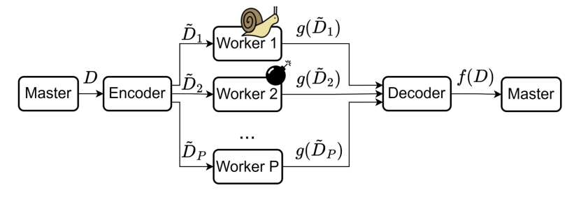
|
|
||||||
|
|
||||||
Matrix-vector multiplication: $y=Ax$, where $A\in \mathbb{F}^{M\times N},x\in \mathbb{F}^N$
|
|
||||||
|
|
||||||
- MDS codes.
|
|
||||||
- Recover threshold $K=M$.
|
|
||||||
- Short-dot codes.
|
|
||||||
- Recover threshold $K\geq M$.
|
|
||||||
- Every node receives at most $s=\frac{P-K+M}{P}$. $N$ elements of $x$.
|
|
||||||
|
|
||||||
### Matrix-matrix multiplication
|
|
||||||
|
|
||||||
Problem Formulation:
|
|
||||||
|
|
||||||
- $A=[A_0 A_1\ldots A_{M-1}]\in \mathbb{F}^{L\times L}$, $B=[B_0,B_1,\ldots,B_{M-1}]\in \mathbb{F}^{L\times L}$
|
|
||||||
- $A_m,B_m$ are submatrices of $A,B$.
|
|
||||||
- We want to compute $C=A^\top B$.
|
|
||||||
|
|
||||||
Trivial solution:
|
|
||||||
|
|
||||||
- Index each worker node by $m,n\in [0,M-1]$.
|
|
||||||
- Worker node $(m,n)$ performs matrix multiplication $A_m^\top\cdot B_n$.
|
|
||||||
- Need $P=M^2$ nodes.
|
|
||||||
- No erasure tolerance.
|
|
||||||
|
|
||||||
Can we do better?
|
|
||||||
|
|
||||||
#### 1-D MDS Method
|
|
||||||
|
|
||||||
Create $[\tilde{A}_0,\tilde{A}_1,\ldots,\tilde{A}_{S-1}]$ by encoding $[A_0,A_1,\ldots,A_{M-1}]$. with some $(S,M)$ MDS code.
|
|
||||||
|
|
||||||
Need $P=SM$ worker nodes, and index each one by $s\in [0,S-1], n\in [0,M-1]$.
|
|
||||||
|
|
||||||
Worker node $(s,n)$ performs matrix multiplication $\tilde{A}_s^\top\cdot B_n$.
|
|
||||||
|
|
||||||
$$
|
|
||||||
\begin{bmatrix}
|
|
||||||
A_0^\top\\
|
|
||||||
A_1^\top\\
|
|
||||||
A_0^\top+A_1^\top
|
|
||||||
\end{bmatrix}
|
|
||||||
\begin{bmatrix}
|
|
||||||
B_0 & B_1
|
|
||||||
\end{bmatrix}
|
|
||||||
$$
|
|
||||||
|
|
||||||
Need $S-M$ responses from each column.
|
|
||||||
|
|
||||||
The recovery threshold $K=P-S+M$ nodes.
|
|
||||||
|
|
||||||
This is trivially parity check code with 1 recovery threshold.
|
|
||||||
|
|
||||||
#### 2-D MDS Method
|
|
||||||
|
|
||||||
Encode $[A_0,A_1,\ldots,A_{M-1}]$ with some $(S,M)$ MDS code.
|
|
||||||
|
|
||||||
Encode $[B_0,B_1,\ldots,B_{M-1}]$ with some $(S,M)$ MDS code.
|
|
||||||
|
|
||||||
Need $P=S^2$ nodes.
|
|
||||||
|
|
||||||
$$
|
|
||||||
\begin{bmatrix}
|
|
||||||
A_0^\top\\
|
|
||||||
A_1^\top\\
|
|
||||||
A_0^\top+A_1^\top
|
|
||||||
\end{bmatrix}
|
|
||||||
\begin{bmatrix}
|
|
||||||
B_0 & B_1 & B_0+B_1
|
|
||||||
\end{bmatrix}
|
|
||||||
$$
|
|
||||||
|
|
||||||
Decodability depends on the pattern.
|
|
||||||
|
|
||||||
- Consider an $S\times S$ bipartite graph (rows on left, columns on right).
|
|
||||||
- Draw an $(i,j)$ edge if $\tilde{A}_i^\top\cdot \tilde{B}_j$ is missing
|
|
||||||
- Row $i$ is decodable if and only if the degree of $i$'th left node $\leq S-M$.
|
|
||||||
- Column $j$ is decodable if and only if the degree of $j$'th right node $\leq S-M$.
|
|
||||||
|
|
||||||
Peeling algorithm:
|
|
||||||
|
|
||||||
- Traverse the graph.
|
|
||||||
- If $\exists v$,$\deg v\leq S-M$, remove edges.
|
|
||||||
- Repeat.
|
|
||||||
|
|
||||||
Corollary:
|
|
||||||
|
|
||||||
- A pattern is decodable if and only if the above graph **does not** contain a subgraph with all degree larger than $S-M$.
|
|
||||||
|
|
||||||
> [!NOTE]
|
|
||||||
>
|
|
||||||
> 1. $K_{1D-MDS}=P-S+M=\Theta(P)$ (linearly)
|
|
||||||
> 2. $K_{2D-MDS}=P-(S-M+1)^2+1$.
|
|
||||||
> - Consider $S\times S$ bipartite graph with $(S-M+1)\times (S-M+1)$ complete subgraph.
|
|
||||||
> - There exists subgraph with all degrees larger than $S-M\implies$ not decodable.
|
|
||||||
> - On the other hand: Fewer than $(S-M+1)^2$ edges cannot form a subgraph with all degrees $>S-M$.
|
|
||||||
> - $K$ scales sub-linearly with $P$.
|
|
||||||
> 3. $K_{product}<P-M^2=S^2-M^2=\Theta(\sqrt{P})$
|
|
||||||
>
|
|
||||||
> Our goal is to get rid of $P$.
|
|
||||||
|
|
||||||
### Polynomial codes
|
|
||||||
|
|
||||||
#### Polynomial representation
|
|
||||||
|
|
||||||
Coefficient representation of a polynomial:
|
|
||||||
|
|
||||||
- $f(x)=f_dx^d+f_{d-1}x^{d-1}+\cdots+f_1x+f_0$
|
|
||||||
- Uniquely defined by coefficients $[f_d,f_{d-1},\ldots,f_0]$.
|
|
||||||
|
|
||||||
Value presentation of a polynomial:
|
|
||||||
|
|
||||||
- Theorem: A polynomial of degree $d$ is uniquely determined by $d+1$ points.
|
|
||||||
- Proof Outline: First create a polynomial of degree $d$ from the $d+1$ points using Lagrange interpolation, and show such polynomial is unique.
|
|
||||||
- Uniquely defined by evaluations $[(\alpha_1,f(\alpha_1)),\ldots,(\alpha_{d},f(\alpha_{d}))]$
|
|
||||||
|
|
||||||
Why should we want value representation?
|
|
||||||
|
|
||||||
- With coefficient representation, polynomial product takes $O(d^2)$ multiplications.
|
|
||||||
- With value representation, polynomial product takes $2d+1$ multiplications.
|
|
||||||
|
|
||||||
#### Definition of a polynomial code
|
|
||||||
|
|
||||||
[link to paper](https://arxiv.org/pdf/1705.10464)
|
|
||||||
|
|
||||||
Problem formulation:
|
|
||||||
|
|
||||||
$$
|
|
||||||
A=[A_0,A_1,\ldots,A_{M-1}]\in \mathbb{F}^{L\times L}, B=[B_0,B_1,\ldots,B_{M-1}]\in \mathbb{F}^{L\times L}
|
|
||||||
$$
|
|
||||||
|
|
||||||
We want to compute $C=A^\top B$.
|
|
||||||
|
|
||||||
Define *matrix* polynomials:
|
|
||||||
|
|
||||||
$p_A(x)=\sum_{i=0}^{M-1} A_i x^i$, degree $M-1$
|
|
||||||
|
|
||||||
$p_B(x)=\sum_{i=0}^{M-1} B_i x^{iM}$, degree $M(M-1)$
|
|
||||||
|
|
||||||
where each $A_i,B_i$ are matrices
|
|
||||||
|
|
||||||
We have
|
|
||||||
|
|
||||||
$$
|
|
||||||
h(x)=p_A(x)p_B(x)=\sum_{i=0}^{M-1}\sum_{j=0}^{M-1} A_i B_j x^{i+jM}
|
|
||||||
$$
|
|
||||||
|
|
||||||
$\deg h(x)\leq M(M-1)+M-1=M^2-1$
|
|
||||||
|
|
||||||
Observe that
|
|
||||||
|
|
||||||
$$
|
|
||||||
x^{i_1+j_1M}=x^{i_2+j_2M}
|
|
||||||
$$
|
|
||||||
if and only if $m_1=n_1$ and $m_2=n_2$.
|
|
||||||
|
|
||||||
The coefficient of $x^{i+jM}$ is $A_i^\top B_j$.
|
|
||||||
|
|
||||||
Computing $C=A^\top B$ is equivalent to find the coefficient representation of $h(x)$.
|
|
||||||
|
|
||||||
#### Encoding of polynomial codes
|
|
||||||
|
|
||||||
The master choose $\omega_0,\omega_1,\ldots,\omega_{P-1}\in \mathbb{F}$.
|
|
||||||
|
|
||||||
- Note that this requires $|\mathbb{F}|\geq P$.
|
|
||||||
|
|
||||||
For every node $i\in [0,P-1]$, the master computes $\tilde{A}_i=p_A(\omega_i)$
|
|
||||||
|
|
||||||
- Equivalent to multiplying $[A_0^\top,A_1^\top,\ldots,A_{M-1}^\top]$ by Vandermonde matrix over $\omega_0,\omega_1,\ldots,\omega_{P-1}$.
|
|
||||||
- Can be speed up using FFT.
|
|
||||||
|
|
||||||
Similarly, the master computes $\tilde{B}_i=p_B(\omega_i)$ for every node $i\in [0,P-1]$.
|
|
||||||
|
|
||||||
Every node $i\in [0,P-1]$ computes and returns $c_i=p_A(\omega_i)p_B(\omega_i)$ to the master.
|
|
||||||
|
|
||||||
$c_i$ is the evaluation of polynomial $h(x)=p_A(x)p_B(x)$ at $\omega_i$.
|
|
||||||
|
|
||||||
Recall that $h(x)=\sum_{i=0}^{M-1}\sum_{j=0}^{M-1} A_i^\top B_j x^{i+jM}$.
|
|
||||||
|
|
||||||
- Computing $C=A^\top B$ is equivalent to finding the coefficient representation of $h(x)$.
|
|
||||||
|
|
||||||
Recall that a polynomial of degree $d$ can be uniquely defined by $d+1$ points.
|
|
||||||
|
|
||||||
- With $MN$ evaluations of $h(x)$, we can recover the coefficient representation for polynomial $h(x)$.
|
|
||||||
|
|
||||||
The recovery threshold $K=M^2$, independent of $P$, the number of worker nodes.
|
|
||||||
|
|
||||||
Done.
|
|
||||||
|
|
||||||
### MatDot Codes
|
|
||||||
|
|
||||||
[link to paper](https://arxiv.org/pdf/1801.10292)
|
|
||||||
|
|
||||||
Problem formulation:
|
|
||||||
|
|
||||||
- We want to compute $C=A^\top B$.
|
|
||||||
- Unlike polynomial codes, we let $A=\begin{bmatrix}
|
|
||||||
A_0\\
|
|
||||||
A_1\\
|
|
||||||
\vdots\\
|
|
||||||
A_{M-1}
|
|
||||||
\end{bmatrix}$ and $B=\begin{bmatrix}
|
|
||||||
B_0\\
|
|
||||||
B_1\\
|
|
||||||
\vdots\\
|
|
||||||
B_{M-1}
|
|
||||||
\end{bmatrix}$. And $A,B\in \mathbb{F}^{L\times L}$.
|
|
||||||
|
|
||||||
- In polynomial codes, $A=\begin{bmatrix}
|
|
||||||
A_0 A_1\ldots A_{M-1}
|
|
||||||
\end{bmatrix}$ and $B=\begin{bmatrix}
|
|
||||||
B_0 B_1\ldots B_{M-1}
|
|
||||||
\end{bmatrix}$.
|
|
||||||
|
|
||||||
Key observation:
|
|
||||||
|
|
||||||
$A_m^\top$ is an $L\times \frac{L}{M}$ matrix, and $B_m$ is an $\frac{L}{M}\times L$ matrix. Hence, $A_m^\top B_m$ is an $L\times L$ matrix.
|
|
||||||
|
|
||||||
Let $C=A^\top B=\sum_{m=0}^{M-1} A_m^\top B_m$.
|
|
||||||
|
|
||||||
Let $p_A(x)=\sum_{m=0}^{M-1} A_m x^m$, degree $M-1$.
|
|
||||||
|
|
||||||
Let $p_B(x)=\sum_{m=0}^{M-1} B_m x^m$, degree $M-1$.
|
|
||||||
|
|
||||||
Both have degree $M-1$.
|
|
||||||
|
|
||||||
And $h(x)=p_A(x)p_B(x)$.
|
|
||||||
|
|
||||||
$\deg h(x)\leq M-1+M-1=2M-2$
|
|
||||||
|
|
||||||
Key observation:
|
|
||||||
|
|
||||||
- The coefficient of the term $x^{M-1}$ in $h(x)$ is $\sum_{m=0}^{M-1} A_m^\top B_m$.
|
|
||||||
|
|
||||||
Recall that $C=A^\top B=\sum_{m=0}^{M-1} A_m^\top B_m$.
|
|
||||||
|
|
||||||
Finding this coefficient is equivalent to finding the result of $A^\top B$.
|
|
||||||
|
|
||||||
> Here we sacrifice the bandwidth of the network for the computational power.
|
|
||||||
|
|
||||||
#### General Scheme for MatDot Codes
|
|
||||||
|
|
||||||
The master choose $\omega_0,\omega_1,\ldots,\omega_{P-1}\in \mathbb{F}$.
|
|
||||||
|
|
||||||
- Note that this requires $|\mathbb{F}|\geq P$.
|
|
||||||
|
|
||||||
For every node $i\in [0,P-1]$, the master computes $\tilde{A}_i=p_A(\omega_i)$ and $\tilde{B}_i=p_B(\omega_i)$.
|
|
||||||
|
|
||||||
- $p_A(x)=\sum_{m=0}^{M-1} A_m x^m$, degree $M-1$.
|
|
||||||
- $p_B(x)=\sum_{m=0}^{M-1} B_m x^m$, degree $M-1$.
|
|
||||||
|
|
||||||
The master sends $\tilde{A}_i,\tilde{B}_i$ to node $i$.
|
|
||||||
|
|
||||||
Every node $i\in [0,P-1]$ computes and returns $c_i=p_A(\omega_i)p_B(\omega_i)$ to the master.
|
|
||||||
|
|
||||||
The master needs $\deg h(x)+1=2M-1$ evaluations to obtain $h(x)$.
|
|
||||||
|
|
||||||
- The recovery threshold is $K=2M-1$
|
|
||||||
|
|
||||||
### Recap on Matrix-Matrix multiplication
|
|
||||||
|
|
||||||
$A,B\in \mathbb{F}^{L\times L}$, we want to compute $C=A^\top B$ with $P$ nodes.
|
|
||||||
|
|
||||||
Every node receives $\frac{1}{m}$ of $A$ and $\frac{1}{m}$ of $B$.
|
|
||||||
|
|
||||||
|Code| Recovery threshold $K$|
|
|
||||||
|:--:|:--:|
|
|
||||||
|1D-MDS| $\Theta(P)$ |
|
|
||||||
|2D-MDS| $\leq \Theta(\sqrt{P})$ |
|
|
||||||
|Polynomial codes| $\Theta(M^2)$ |
|
|
||||||
|MatDot codes| $\Theta(M)$ |
|
|
||||||
|
|
||||||
## Polynomial Evaluation
|
|
||||||
|
|
||||||
Problem formulation:
|
|
||||||
|
|
||||||
- We have $K$ datasets $X_1,X_2,\ldots,X_K$.
|
|
||||||
- Want to compute some polynomial function $f$ of degree $d$ on each dataset.
|
|
||||||
- Want $f(X_1),f(X_2),\ldots,f(X_K)$.
|
|
||||||
- Examples:
|
|
||||||
- $X_1,X_2,\ldots,X_K$ are points in $\mathbb{F}^{M\times M}$, and $f(X)=X^8+3X^2+1$.
|
|
||||||
- $X_k=(X_k^{(1)},X_k^{(2)})$, both in $\mathbb{F}^{M\times M}$, and $f(X)=X_k^{(1)}X_k^{(2)}$.
|
|
||||||
- Gradient computation.
|
|
||||||
|
|
||||||
$P$ worker nodes:
|
|
||||||
|
|
||||||
- Some are stragglers, i.e., not responsive.
|
|
||||||
- Some are adversaries, i.e., return erroneous results.
|
|
||||||
- Privacy: We do not want to expose datasets to worker nodes.
|
|
||||||
|
|
||||||
### Replication code
|
|
||||||
|
|
||||||
Suppose $P=(r+1)\cdot K$.
|
|
||||||
|
|
||||||
- Partition the $P$ nodes to $K$ groups of size $r+1$ each.
|
|
||||||
- Node in group $i$ computes and returns $f(X_i)$ to the master.
|
|
||||||
- Replication tolerates $r$ stragglers, or $\lfloor \frac{r}{2} \rfloor$ adversaries.
|
|
||||||
|
|
||||||
### Linear codes
|
|
||||||
|
|
||||||
Recall previous linear computations (matrix-vector):
|
|
||||||
|
|
||||||
- $[\tilde{A}_1,\tilde{A}_2,\tilde{A}_3]=[A_1,A_2,A_1+A_2]$ is the corresponding codeword of $[A_1,A_2]$.
|
|
||||||
- Every worker node $i$ computes $f(\tilde{A}_i)=\tilde{A}_i x$.
|
|
||||||
- $[\tilde{A}_1x, \tilde{A}_2x, \tilde{A}_3x]=[A_1x,A_2x,A_1x+A_2x]$ is the corresponding codeword of $[A_1x,A_2x]$.
|
|
||||||
- This enables to decode $[A_1x,A_2x]$ from $[\tilde{A}_1x,\tilde{A}_2x,\tilde{A}_3 x]$.
|
|
||||||
|
|
||||||
However, $f$ is a **polynomial of degree $d$**, not a linear transformation unless $d=1$.
|
|
||||||
|
|
||||||
- $f(cX)\neq cf(X)$, where $c$ is a constant.
|
|
||||||
- $f(X_1+X_2)\neq f(X_1)+f(X_2)$.
|
|
||||||
|
|
||||||
> [!CAUTION]
|
|
||||||
>
|
|
||||||
> $[f(\tilde{X}_1),f(\tilde{X}_2),\ldots,f(\tilde{X}_K)]$ is not the codeword corresponding to $[f(X_1),f(X_2),\ldots,f(X_K)]$ in any linear code.
|
|
||||||
|
|
||||||
Our goal is to create an encoder/decode such that:
|
|
||||||
|
|
||||||
- Linear encoding: is the codeword of $[X_1,X_2,\ldots,X_K]$ for some linear code.
|
|
||||||
- i.e., $[\tilde{X}_1,\tilde{X}_2,\ldots,\tilde{X}_K]=[X_1,X_2,\ldots,X_K]G$ for some generator matrix $G$.
|
|
||||||
- Every $\tilde{X}_i$ is some linear combination of $X_1,\ldots,X_K$.
|
|
||||||
- The $f(X_i)$ are decodable from some subset of $f(\tilde{X}_i)$'s.
|
|
||||||
- Some of coded results are missing, erroneous.
|
|
||||||
- $X_i$'s are kept private.
|
|
||||||
|
|
||||||
### Lagrange Coded Computing
|
|
||||||
|
|
||||||
Let $\ell(z)$ be a polynomial whose evaluations at $\omega_1,\ldots,\omega_{K}$ are $X_1,\ldots,X_K$.
|
|
||||||
|
|
||||||
- That is, $\ell(\omega_i)=X_i$ for every $\omega_i\in \mathbb{F}, i\in [K]$.
|
|
||||||
|
|
||||||
Some example constructions:
|
|
||||||
|
|
||||||
Given $X_1,\ldots,X_K$ with corresponding $\omega_1,\ldots,\omega_K$
|
|
||||||
|
|
||||||
- $\ell(z)=\sum_{i=1}^K X_iL_i(z)$, where $L_i(z)=\prod_{j\in[K],j\neq i} \frac{z-\omega_j}{\omega_i-\omega_j}=\begin{cases} 0 & \text{if } j\neq i \\ 1 & \text{if } j=i \end{cases}$.
|
|
||||||
|
|
||||||
Then every $f(X_i)=f(\ell(\omega_i))$ is an evaluation of polynomial $f\circ \ell(z)$ at $\omega_i$.
|
|
||||||
|
|
||||||
If the master obtains the composition $h=f\circ \ell$, it can obtain every $f(X_i)=h(\omega_i)$.
|
|
||||||
|
|
||||||
Goal: The master wished to obtain the polynomial $h(z)=f(\ell(z))$.
|
|
||||||
|
|
||||||
Intuition:
|
|
||||||
|
|
||||||
- Encoding is performed by evaluating $\ell(z)$ at $\alpha_1,\ldots,\alpha_P\in \mathbb{F}$, and $P>K$ for redundancy.
|
|
||||||
- Nodes apply $f$ on an evaluation of $\ell$ and obtain an evaluation of $h$.
|
|
||||||
- The master receives some potentially noisy evaluations, and finds $h$.
|
|
||||||
- The master evaluates $h$ at $\omega_1,\ldots,\omega_K$ to obtain $f(X_1),\ldots,f(X_K)$.
|
|
||||||
|
|
||||||
### Encoding for Lagrange coded computing
|
|
||||||
|
|
||||||
Need polynomial $\ell(z)$ such that:
|
|
||||||
|
|
||||||
- $X_k=\ell(\omega_k)$ for every $k\in [K]$.
|
|
||||||
|
|
||||||
Having obtained such $\ell$ we let $\tilde{X}_i=\ell(\alpha_i)$ for every $i\in [P]$.
|
|
||||||
|
|
||||||
$span{\tilde{X}_1,\tilde{X}_2,\ldots,\tilde{X}_P}=span{\ell_1(x),\ell_2(x),\ldots,\ell_P(x)}$.
|
|
||||||
|
|
||||||
Want $X_k=\ell(\omega_k)$ for every $k\in [K]$.
|
|
||||||
|
|
||||||
Tool: Lagrange interpolation.
|
|
||||||
|
|
||||||
- $\ell_k(z)=\prod_{i\neq k} \frac{z-\omega_j}{\omega_k-\omega_j}$.
|
|
||||||
- $\ell_k(\omega_k)=1$ and $\ell_k(\omega_k)=0$ for every $j\neq k$.
|
|
||||||
- $\deg \ell_k(z)=K-1$.
|
|
||||||
|
|
||||||
Let $\ell(z)=\sum_{k=1}^K X_k\ell_k(z)$.
|
|
||||||
|
|
||||||
- $\deg \ell\leq K-1$.
|
|
||||||
- $\ell(\omega_k)=X_k$ for every $k\in [K]$.
|
|
||||||
|
|
||||||
Let $\tilde{X}_i=\ell(\alpha_i)=\sum_{k=1}^K X_k\ell_k(\alpha_i)$.
|
|
||||||
|
|
||||||
Every $\tilde{X}_i$ is a **linear combination** of $X_1,\ldots,X_K$.
|
|
||||||
|
|
||||||
$$
|
|
||||||
(\tilde{X}_1,\tilde{X}_2,\ldots,\tilde{X}_P)=(X_1,\ldots,X_K)\cdot G=(X_1,\ldots,X_K)\begin{bmatrix}
|
|
||||||
\ell_1(\alpha_1) & \ell_1(\alpha_2) & \cdots & \ell_1(\alpha_P) \\
|
|
||||||
\ell_2(\alpha_1) & \ell_2(\alpha_2) & \cdots & \ell_2(\alpha_P) \\
|
|
||||||
\vdots & \vdots & \ddots & \vdots \\
|
|
||||||
\ell_K(\alpha_1) & \ell_K(\alpha_2) & \cdots & \ell_K(\alpha_P)
|
|
||||||
\end{bmatrix}
|
|
||||||
$$
|
|
||||||
|
|
||||||
This $G$ is called a **Lagrange matrix** with respect to
|
|
||||||
|
|
||||||
- $\omega_1,\ldots,\omega_K$. (interpolation points)
|
|
||||||
- $\alpha_1,\ldots,\alpha_P$. (evaluation points)
|
|
||||||
|
|
||||||
> Continue next lecture
|
|
||||||
@@ -1,327 +0,0 @@
|
|||||||
# CSE5313 Coding and information theory for data science (Lecture 25)
|
|
||||||
|
|
||||||
## Polynomial Evaluation
|
|
||||||
|
|
||||||
Problem formulation:
|
|
||||||
|
|
||||||
- We have $K$ datasets $X_1,X_2,\ldots,X_K$.
|
|
||||||
- Want to compute some polynomial function $f$ of degree $d$ on each dataset.
|
|
||||||
- Want $f(X_1),f(X_2),\ldots,f(X_K)$.
|
|
||||||
- Examples:
|
|
||||||
- $X_1,X_2,\ldots,X_K$ are points in $\mathbb{F}^{M\times M}$, and $f(X)=X^8+3X^2+1$.
|
|
||||||
- $X_k=(X_k^{(1)},X_k^{(2)})$, both in $\mathbb{F}^{M\times M}$, and $f(X)=X_k^{(1)}X_k^{(2)}$.
|
|
||||||
- Gradient computation.
|
|
||||||
|
|
||||||
$P$ worker nodes:
|
|
||||||
|
|
||||||
- Some are stragglers, i.e., not responsive.
|
|
||||||
- Some are adversaries, i.e., return erroneous results.
|
|
||||||
- Privacy: We do not want to expose datasets to worker nodes.
|
|
||||||
|
|
||||||
### Lagrange Coded Computing
|
|
||||||
|
|
||||||
Let $\ell(z)$ be a polynomial whose evaluations at $\omega_1,\ldots,\omega_{K}$ are $X_1,\ldots,X_K$.
|
|
||||||
|
|
||||||
- That is, $\ell(\omega_i)=X_i$ for every $\omega_i\in \mathbb{F}, i\in [K]$.
|
|
||||||
|
|
||||||
Some example constructions:
|
|
||||||
|
|
||||||
Given $X_1,\ldots,X_K$ with corresponding $\omega_1,\ldots,\omega_K$
|
|
||||||
|
|
||||||
- $\ell(z)=\sum_{i=1}^K X_i\ell_i(z)$, where $\ell_i(z)=\prod_{j\in[K],j\neq i} \frac{z-\omega_j}{\omega_i-\omega_j}=\begin{cases} 0 & \text{if } j\neq i \\ 1 & \text{if } j=i \end{cases}$.
|
|
||||||
|
|
||||||
Then every $f(X_i)=f(\ell(\omega_i))$ is an evaluation of polynomial $f\circ \ell(z)$ at $\omega_i$.
|
|
||||||
|
|
||||||
If the master obtains the composition $h=f\circ \ell$, it can obtain every $f(X_i)=h(\omega_i)$.
|
|
||||||
|
|
||||||
Goal: The master wished to obtain the polynomial $h(z)=f(\ell(z))$.
|
|
||||||
|
|
||||||
Intuition:
|
|
||||||
|
|
||||||
- Encoding is performed by evaluating $\ell(z)$ at $\alpha_1,\ldots,\alpha_P\in \mathbb{F}$, and $P>K$ for redundancy.
|
|
||||||
- Nodes apply $f$ on an evaluation of $\ell$ and obtain an evaluation of $h$.
|
|
||||||
- The master receives some potentially noisy evaluations, and finds $h$.
|
|
||||||
- The master evaluates $h$ at $\omega_1,\ldots,\omega_K$ to obtain $f(X_1),\ldots,f(X_K)$.
|
|
||||||
|
|
||||||
### Encoding for Lagrange coded computing
|
|
||||||
|
|
||||||
Need polynomial $\ell(z)$ such that:
|
|
||||||
|
|
||||||
- $X_k=\ell(\omega_k)$ for every $k\in [K]$.
|
|
||||||
|
|
||||||
Having obtained such $\ell$ we let $\tilde{X}_i=\ell(\alpha_i)$ for every $i\in [P]$.
|
|
||||||
|
|
||||||
$span{\tilde{X}_1,\tilde{X}_2,\ldots,\tilde{X}_P}=span{\ell_1(x),\ell_2(x),\ldots,\ell_P(x)}$.
|
|
||||||
|
|
||||||
Want $X_k=\ell(\omega_k)$ for every $k\in [K]$.
|
|
||||||
|
|
||||||
Tool: Lagrange interpolation.
|
|
||||||
|
|
||||||
- $\ell_k(z)=\prod_{i\neq k} \frac{z-\omega_j}{\omega_k-\omega_j}$.
|
|
||||||
- $\ell_k(\omega_k)=1$ and $\ell_k(\omega_k)=0$ for every $j\neq k$.
|
|
||||||
- $\deg \ell_k(z)=K-1$.
|
|
||||||
|
|
||||||
Let $\ell(z)=\sum_{k=1}^K X_k\ell_k(z)$.
|
|
||||||
|
|
||||||
- $\deg \ell\leq K-1$.
|
|
||||||
- $\ell(\omega_k)=X_k$ for every $k\in [K]$.
|
|
||||||
|
|
||||||
Let $\tilde{X}_i=\ell(\alpha_i)=\sum_{k=1}^K X_k\ell_k(\alpha_i)$.
|
|
||||||
|
|
||||||
Every $\tilde{X}_i$ is a **linear combination** of $X_1,\ldots,X_K$.
|
|
||||||
|
|
||||||
$$
|
|
||||||
(\tilde{X}_1,\tilde{X}_2,\ldots,\tilde{X}_P)=(X_1,\ldots,X_K)\cdot G=(X_1,\ldots,X_K)\begin{bmatrix}
|
|
||||||
\ell_1(\alpha_1) & \ell_1(\alpha_2) & \cdots & \ell_1(\alpha_P) \\
|
|
||||||
\ell_2(\alpha_1) & \ell_2(\alpha_2) & \cdots & \ell_2(\alpha_P) \\
|
|
||||||
\vdots & \vdots & \ddots & \vdots \\
|
|
||||||
\ell_K(\alpha_1) & \ell_K(\alpha_2) & \cdots & \ell_K(\alpha_P)
|
|
||||||
\end{bmatrix}
|
|
||||||
$$
|
|
||||||
|
|
||||||
This $G$ is called a **Lagrange matrix** with respect to
|
|
||||||
|
|
||||||
- $\omega_1,\ldots,\omega_K$. (interpolation points, rows)
|
|
||||||
- $\alpha_1,\ldots,\alpha_P$. (evaluation points, columns)
|
|
||||||
|
|
||||||
> Basically, a modification of Reed-Solomon code.
|
|
||||||
|
|
||||||
### Decoding for Lagrange coded computing
|
|
||||||
|
|
||||||
Say the system has $S$ stragglers (erasures) and $A$ adversaries (errors).
|
|
||||||
|
|
||||||
The master receives $P-S$ computation results $f(\tilde{X}_{i_1}),\ldots,f(\tilde{X}_{i_{P-S}})$.
|
|
||||||
|
|
||||||
- By design, therese are evaluations of $h: h(a_{i_1})=f(\ell(a_{i_1})),\ldots,h(a_{i_{P-S}})=f(\ell(a_{i_{P-S}}))$
|
|
||||||
- A evaluation are noisy
|
|
||||||
- $\deg h=\deg f\cdot \deg \ell=(K-1)\deg f$.
|
|
||||||
|
|
||||||
Which process enables to interpolate a polynomial from noisy evaluations?
|
|
||||||
|
|
||||||
Ree-Solomon (RS) decoding.
|
|
||||||
|
|
||||||
Fact: Reed-Solomon decoding succeeds if and only if the number of erasures + 2 $\times$ the number of errors $\leq d-1$.
|
|
||||||
|
|
||||||
Imagine $h$ as the "message" in Reed-Solomon code. $[P,(K-1)\deg f +1,P-(K-1)\deg f]_q$.
|
|
||||||
|
|
||||||
- Interpolating $h$ is possible if and only if $S+2A\leq (K-1)\deg f-1$.
|
|
||||||
|
|
||||||
Once the master interpolates $h$.
|
|
||||||
|
|
||||||
- The evaluations $h(\omega_i)=f(\ell(\omega_i))=f(X_i)$ provides the interpolation results.
|
|
||||||
|
|
||||||
#### Theorem of Lagrange coded computing
|
|
||||||
|
|
||||||
Lagrange coded computing enables to compute $\{f(X_i)\}_{i=1}^K$ for any $f$ at the presence of at most $S$ stragglers and at most $A$ adversaries if
|
|
||||||
|
|
||||||
$$
|
|
||||||
(K-1)\deg f+S+2A+1\leq P
|
|
||||||
$$
|
|
||||||
|
|
||||||
> Interpolation of result does not depend on $P$ (number of worker nodes).
|
|
||||||
|
|
||||||
### Privacy for Lagrange coded computing
|
|
||||||
|
|
||||||
Currently any size-$K$ group of colluding nodes reveals the entire dataset.
|
|
||||||
|
|
||||||
Q: Can an individual node $i$ learn anything about $X_i$?
|
|
||||||
|
|
||||||
A: Yes, since $\tilde{X}_i$ is a linear combination of $X_1,\ldots,X_K$ (partial knowledge, a linear combination of private data).
|
|
||||||
|
|
||||||
Can we provide **perfect privacy** given that at most $T$ nodes collude?
|
|
||||||
|
|
||||||
- That is, $I(X:\tilde{X}_i)=0$ for every $\mathcal{T}\subseteq [P]$ of size at most $T$, where
|
|
||||||
- $X=(X_1,\ldots,X_K)$, and
|
|
||||||
- $\tilde{X}_\mathcal{T}=(\tilde{X}_{i_1},\ldots,\tilde{X}_{i_{|\mathcal{T}|}})$.
|
|
||||||
|
|
||||||
Solution: Slight change of encoding in LLC.
|
|
||||||
|
|
||||||
This only applied to $\mathbb{F}=\mathbb{F}_q$ (no perfect privacy over $\mathbb{R},\mathbb{C}$. No uniform distribution can be defined).
|
|
||||||
|
|
||||||
The master chooses
|
|
||||||
|
|
||||||
- $T$ keys $Z_{K+1},\ldots,Z_{K+T}$ uniformly at random ($|Z_i|=|X_i|$ for all $i$)
|
|
||||||
- Interpolation points $\omega_1,\ldots,\omega_{K+T}$.
|
|
||||||
|
|
||||||
Find the Lagrange polynomial $\ell(z)$ such that
|
|
||||||
|
|
||||||
- $\ell(w_i)=X_i$ for $i\in [K]$
|
|
||||||
- $\ell(w_{K+j})=Z_j$ for $j\in [T]$.
|
|
||||||
|
|
||||||
Lagrange interpolation:
|
|
||||||
|
|
||||||
$$
|
|
||||||
\ell(z)=\sum_{i=1}^{K} X_i\ell_i(z)+\sum_{j=1}^{T} X_{K+j}ell_{K+j}(z)
|
|
||||||
$$
|
|
||||||
|
|
||||||
$$
|
|
||||||
(\tilde{X}_1,\ldots,\tilde{X}_P)=(X_1,\ldots,X_K,Z_1,\ldots,Z_T)\cdot G
|
|
||||||
$$
|
|
||||||
|
|
||||||
where
|
|
||||||
|
|
||||||
$$
|
|
||||||
G=\begin{bmatrix}
|
|
||||||
\ell_1(\alpha_1) & \ell_1(\alpha_2) & \cdots & \ell_1(\alpha_P) \\
|
|
||||||
\ell_2(\alpha_1) & \ell_2(\alpha_2) & \cdots & \ell_2(\alpha_P) \\
|
|
||||||
\vdots & \vdots & \ddots & \vdots \\
|
|
||||||
\ell_K(\alpha_1) & \ell_K(\alpha_2) & \cdots & \ell_K(\alpha_P) \\
|
|
||||||
\vdots & \vdots & \ddots & \vdots \\
|
|
||||||
\ell_{K+T}(\alpha_1) & \ell_{K+T}(\alpha_2) & \cdots & \ell_{K+T}(\alpha_P)
|
|
||||||
\end{bmatrix}
|
|
||||||
$$
|
|
||||||
|
|
||||||
For analysis, we denote $G=\begin{bmatrix}G^{top}\\G^{bot}\end{bmatrix}$, where $G^{top}\in \mathbb{F}^{K\times P}$ and $G^{bot}\in \mathbb{F}^{T\times P}$.
|
|
||||||
|
|
||||||
The proof for privacy is the almost the same as ramp scheme.
|
|
||||||
|
|
||||||
<details>
|
|
||||||
<summary>Proof</summary>
|
|
||||||
|
|
||||||
We have $(\tilde{X}_1,\ldots \tilde{X}_P)=(X_1,\ldots,X_K)\cdot G^{top}+(Z_1,\ldots,Z_T)\cdot G^{bot}$.
|
|
||||||
|
|
||||||
Without loss of generality, $\mathcal{T}=[T]$ is the colluding set.
|
|
||||||
|
|
||||||
$\mathcal{T}$ hold $(\tilde{X}_1,\ldots \tilde{X}_P)=(X_1,\ldots,X_K)\cdot G^{top}_\mathcal{T}+(Z_1,\ldots,Z_T)\cdot G^{bot}_\mathcal{top}$.
|
|
||||||
|
|
||||||
- $G^{top}_\mathcal{T}$, $G^{bot}_\mathcal{T}$ contain the first $T$ columns of $G^{top}$, $G^{bot}$, respectively.
|
|
||||||
|
|
||||||
Note that $G^{top}\in \mathbb{F}^{T\times P}_q$ is MDS, and hence $G^{top}_\mathcal{T}$ is a $T\times T$ invertible matrix.
|
|
||||||
|
|
||||||
Since $Z=(Z_1,\ldots,Z_T)$ chosen uniformly random, so $Z\cdot G^{bot}_\mathcal{T}$ is a one-time pad.
|
|
||||||
|
|
||||||
Same proof for decoding, we only need $K+1$ item to make the interpolation work.
|
|
||||||
|
|
||||||
</details>
|
|
||||||
|
|
||||||
## Conclusion
|
|
||||||
|
|
||||||
- Theorem: Lagrange Coded Computing is resilient against $S$ stragglers, $A$ adversaries, and $T$ colluding nodes if
|
|
||||||
$$
|
|
||||||
P\geq (K+T-1)\deg f+S+2A+1
|
|
||||||
$$
|
|
||||||
- Privacy (increase with $\deg f$) cost more than the straggler and adversary (increase linearly).
|
|
||||||
- Caveat: Requires finite field arithmetic!
|
|
||||||
- Some follow-up works analyzed information leakage over the reals
|
|
||||||
|
|
||||||
## Side note for Blockchain
|
|
||||||
|
|
||||||
Blockchain: A decentralized system for trust management.
|
|
||||||
|
|
||||||
Blockchain maintains a chain of blocks.
|
|
||||||
|
|
||||||
- A block contains a set of transactions.
|
|
||||||
- Transaction = value transfer between clients.
|
|
||||||
- The chain is replicated on each node.
|
|
||||||
|
|
||||||
Periodically, a new block is proposed and appended to each local chain.
|
|
||||||
|
|
||||||
- The block must not contain invalid transactions.
|
|
||||||
- Nodes must agree on proposed block.
|
|
||||||
|
|
||||||
Existing systems:
|
|
||||||
|
|
||||||
- All nodes perform the same set of tasks.
|
|
||||||
- Every node must receive every block.
|
|
||||||
|
|
||||||
Performance does not scale with number of node
|
|
||||||
|
|
||||||
### Improving performance of blockchain
|
|
||||||
|
|
||||||
The performance of blockchain is inherently limited by its design.
|
|
||||||
|
|
||||||
- All nodes perform the same set of tasks.
|
|
||||||
- Every node must receive every block.
|
|
||||||
|
|
||||||
Idea: Combine blockchain with distributed computing.
|
|
||||||
|
|
||||||
- Node tasks should complement each other.
|
|
||||||
|
|
||||||
Sharding (notion from databases):
|
|
||||||
|
|
||||||
- Nodes are partitioned into groups of equal size.
|
|
||||||
- Each group maintains a local chain.
|
|
||||||
- More nodes, more groups, more transactions can be processed.
|
|
||||||
- Better performance.
|
|
||||||
|
|
||||||
### Security Problem
|
|
||||||
|
|
||||||
Biggest problem in blockchains: Adversarial (Byzantine) nodes.
|
|
||||||
|
|
||||||
- Malicious actors wish to include invalid transactions.
|
|
||||||
|
|
||||||
Solution in traditional blockchains: Consensus mechanisms.
|
|
||||||
|
|
||||||
- Algorithms for decentralized agreement.
|
|
||||||
- Tolerates up to $1/3$ Byzantine nodes.
|
|
||||||
|
|
||||||
Problem: Consensus conflicts with sharding.
|
|
||||||
|
|
||||||
- Traditional consensus mechanisms tolerate $\approx 1/3$ Byzantine nodes.
|
|
||||||
- If we partition $P$ nodes into $K$ groups, we can tolerate only $P/3K$ node failures.
|
|
||||||
- Down from $P/3$ in non-shared systems.
|
|
||||||
|
|
||||||
Goal: Solve the consensus problem in sharded systems.
|
|
||||||
|
|
||||||
Tool: Coded computing.
|
|
||||||
|
|
||||||
### Problem formulation
|
|
||||||
|
|
||||||
At epoch $t$ of a shared blockchain system, we have
|
|
||||||
|
|
||||||
- $K$ local chain $Y_1^{t-1},\ldots, Y_K^{t-1}$.
|
|
||||||
- $K$ new blocks $X_1(t),\ldots,X_K(t)$.
|
|
||||||
- A polynomial verification function $f(X_k(t),Y_k^t)$, which validates $X_k(t)$.
|
|
||||||
|
|
||||||
<details>
|
|
||||||
<summary>Proof</summary>
|
|
||||||
|
|
||||||
Balance check function $f(X_k(t),Y_k^t)=\sum_\tau Y_k(\tau)-X_k(t)$.
|
|
||||||
|
|
||||||
More commonly, a (polynomial) hash function. Used to:
|
|
||||||
|
|
||||||
- Verify the sender's public key.
|
|
||||||
- Verify the ownership of the transferred funds.
|
|
||||||
|
|
||||||
</details>
|
|
||||||
|
|
||||||
Need: Apply a polynomial functions on $K$ datasets.
|
|
||||||
|
|
||||||
Lagrange coded computing!
|
|
||||||
|
|
||||||
### Blockchain with Lagrange coded computing
|
|
||||||
|
|
||||||
At epoch $t$:
|
|
||||||
|
|
||||||
- A leader is elected (using secure election mechanism).
|
|
||||||
- The leader receives new blocks $X_1(t),\ldots,X_K(t)$.
|
|
||||||
- The leader disperses the encoded blocks $\tilde{X}_1(t),\ldots,\tilde{X}_P(t)$ to nodes.
|
|
||||||
- Needs secure information dispersal mechanisms.
|
|
||||||
|
|
||||||
Every node $i\in [P]$:
|
|
||||||
|
|
||||||
- Locally stores a coded chain $\tilde{Y}_i^t$ (encoded using LCC).
|
|
||||||
- Receives $\tilde{X}_i(t)$.
|
|
||||||
- Computes $f(\tilde{X}_i(t),\tilde{Y}_i^t)$ and sends to the leader.
|
|
||||||
|
|
||||||
The leader decodes to get $\{f(X_i(t),Y_i^t)\}_{i=1}^K$ and disperse securely to nodes.
|
|
||||||
|
|
||||||
Node $i$ appends coded block $\tilde{X}_i(t)$ to coded chain $\tilde{Y}_i^t$ (zeroing invalid transactions).
|
|
||||||
|
|
||||||
Guarantees security if $P\geq (K+T-1)\deg f+S+2A+1$.
|
|
||||||
|
|
||||||
- $A$ adversaries, degree $d$ verification polynomial.
|
|
||||||
|
|
||||||
Sharding without sharding:
|
|
||||||
|
|
||||||
- Computations are done on (coded) partial chains/blocks.
|
|
||||||
- Good performance!
|
|
||||||
- Since blocks/chains are coded, they are "dispersed" among many nodes.
|
|
||||||
- Security problem in sharding solved!
|
|
||||||
- Since the encoding is done (securely) through a leader, no need to send every block to all nodes.
|
|
||||||
- Reduced communication! (main bottleneck).
|
|
||||||
|
|
||||||
Novelties:
|
|
||||||
|
|
||||||
- First decentralized verification system with less than size of blocks times the number of nodes communication.
|
|
||||||
- Coded consensus – Reach consensus on coded data.
|
|
||||||
@@ -1,445 +0,0 @@
|
|||||||
# CSE5313 Coding and information theory for data science (Lecture 26)
|
|
||||||
|
|
||||||
## Sliced and Broken Information with applications in DNA storage and 3D printing
|
|
||||||
|
|
||||||
### Basic info
|
|
||||||
|
|
||||||
Deoxyribo-Nucleic Acid.
|
|
||||||
|
|
||||||
A double-helix shaped molecule.
|
|
||||||
|
|
||||||
Each helix is a string of
|
|
||||||
|
|
||||||
- Cytosine,
|
|
||||||
- Guanine,
|
|
||||||
- Adenine, and
|
|
||||||
- Thymine.
|
|
||||||
|
|
||||||
Contained inside every living cell.
|
|
||||||
|
|
||||||
- Inside the nucleus.
|
|
||||||
|
|
||||||
Used to encode proteins.
|
|
||||||
|
|
||||||
mRNA carries info to Ribosome as codons of length 3 over GUCA.
|
|
||||||
|
|
||||||
- Each codon produces an amino acids.
|
|
||||||
- $4^3> 20$, redundancy in nature!
|
|
||||||
|
|
||||||
1st Chargaff rule:
|
|
||||||
|
|
||||||
- The two strands are complements (A-T and G-C).
|
|
||||||
- $#A = #T$ and $#G = #C$ in both strands.
|
|
||||||
|
|
||||||
2nd Chargaff rule:
|
|
||||||
|
|
||||||
- $#A \approx #T$ and $#G \approx #C$ in each strands.
|
|
||||||
- Can be explained via tandem duplications.
|
|
||||||
- $GCAGCATT \implies GCAGCAGCATT$.
|
|
||||||
- Occur naturally during cell mitosis.
|
|
||||||
|
|
||||||
### DNA storage
|
|
||||||
|
|
||||||
DNA synthesis:
|
|
||||||
|
|
||||||
- Artificial creation of DNA from G’s, T’s, A’s, and C’s.
|
|
||||||
|
|
||||||
Can be used to store information!
|
|
||||||
|
|
||||||
Advantages:
|
|
||||||
|
|
||||||
- Density.
|
|
||||||
- 5.5 PB per mm3.
|
|
||||||
- Stability.
|
|
||||||
- Half-life 521 years (compare to ≈ 20𝑦 on hard drives).
|
|
||||||
- Future proof.
|
|
||||||
- DNA reading and writing will remain relevant "forever."
|
|
||||||
|
|
||||||
#### DNA storage prototypes
|
|
||||||
|
|
||||||
Some recent attempts:
|
|
||||||
|
|
||||||
- 2011, 659kb.
|
|
||||||
- Church, Gao, Kosuri, "Next-generation digital information storage in DNA", Science.
|
|
||||||
- 2018, 200MB.
|
|
||||||
- Organick et al., "Random access in large-scale DNA data storage," Nature biotechnology.
|
|
||||||
- CatalogDNA (startup):
|
|
||||||
- 2019, 16GB.
|
|
||||||
- 2021, 18 Mbps.
|
|
||||||
|
|
||||||
Companies:
|
|
||||||
|
|
||||||
- Microsoft, Illumina, Western Digital, many startups.
|
|
||||||
|
|
||||||
Challenges:
|
|
||||||
|
|
||||||
- Expensive, Slow.
|
|
||||||
- Traditional storage media still sufficient and affordable.
|
|
||||||
|
|
||||||
#### DNA Storage models
|
|
||||||
|
|
||||||
In vivo:
|
|
||||||
|
|
||||||
- Implant the synthetic DNA inside a living organism.
|
|
||||||
- Need evolution-correcting codes!
|
|
||||||
- E.g., coding against tandem-duplications.
|
|
||||||
|
|
||||||
In vitro:
|
|
||||||
|
|
||||||
- Place the synthetic DNA in test tubes.
|
|
||||||
- Challenge: Can only synthesize short sequences ($\approx 1000 bp$).
|
|
||||||
- 1 test tube contains millions to billions of short sequences.
|
|
||||||
|
|
||||||
How to encode information?
|
|
||||||
|
|
||||||
How to achieve noise robustness?
|
|
||||||
|
|
||||||
### DNA coding in vitro environment
|
|
||||||
|
|
||||||
Traditional data communication:
|
|
||||||
|
|
||||||
$$
|
|
||||||
m\in\{0,1\}^k\mapsto c\in\{0,1\}^n
|
|
||||||
$$
|
|
||||||
|
|
||||||
DNA storage:
|
|
||||||
|
|
||||||
$$
|
|
||||||
m\in\{0,1\}^k\mapsto c\in \binom{\{0,1\}^L}{M}
|
|
||||||
$$
|
|
||||||
|
|
||||||
where $\binom{\{0,1\}^L}{M}$ is the collection of all $M$-subsets of $\{0,1\}^L$. ($0\leq M\leq 2^L$)
|
|
||||||
|
|
||||||
A codeword is a set of $M$ binary strings, each of length $L$.
|
|
||||||
|
|
||||||
"Sliced channel":
|
|
||||||
|
|
||||||
- The message $m$ is encoded to $c\in \{0,1\}^{ML}, and then sliced to $M$ equal parts.
|
|
||||||
- Parts may be noisy (substitutions, deletions, etc.).
|
|
||||||
- Also useful in network packet transmission ($M$ packets of length $L$).
|
|
||||||
|
|
||||||
#### Sliced channel: Figures of merit
|
|
||||||
|
|
||||||
How to quantify the **merit** of a given code $\mathcal{C}$?
|
|
||||||
|
|
||||||
- Want resilience to any $K$ substitutions in all $M$ parts.
|
|
||||||
|
|
||||||
Redundance:
|
|
||||||
|
|
||||||
- Recall in linear codes,
|
|
||||||
- $redundancy=length-dimension=\log (size\ of\ space)-\log (size\ of\ code)$.
|
|
||||||
- In sliced channel:
|
|
||||||
- $redundancy=\log (size\ of\ space)-\log (size\ of\ code)=\log \binom{2^L}{M}-\log |\mathcal{C}|$.
|
|
||||||
|
|
||||||
Research questions:
|
|
||||||
|
|
||||||
- Bounds on redundancy?
|
|
||||||
- Code construction?
|
|
||||||
- Is more redundancy needed in sliced channel?
|
|
||||||
|
|
||||||
#### Sliced channel: Lower bound
|
|
||||||
|
|
||||||
Idea: **Sphere packing**
|
|
||||||
|
|
||||||
Given $c\in \binom{\{0,1\}^L}{M}$ and $K=1$, how may codewords must we exclude?
|
|
||||||
|
|
||||||
<details>
|
|
||||||
<summary>Example</summary>
|
|
||||||
|
|
||||||
- $L=3,M=2$, and let $c=\{001,011\}$. Ball of radius 1 is sized 5.
|
|
||||||
|
|
||||||
all the codeword with distance 1 from $c$ are:
|
|
||||||
|
|
||||||
Distance 0:
|
|
||||||
|
|
||||||
$$
|
|
||||||
\{001,011\}
|
|
||||||
$$
|
|
||||||
|
|
||||||
Distance 1:
|
|
||||||
$$
|
|
||||||
\{101,011\}\quad \{011\}\quad \{000,011\}\\
|
|
||||||
\{001,111\}\quad \{001\}\quad \{001,010\}
|
|
||||||
$$
|
|
||||||
|
|
||||||
7 options and 2 of them are not codewords.
|
|
||||||
|
|
||||||
So the effective size of the ball is 5.
|
|
||||||
|
|
||||||
</details>
|
|
||||||
|
|
||||||
Tool: (Fourier analysis of) Boolean functions
|
|
||||||
|
|
||||||
Introducing hypercube graph:
|
|
||||||
|
|
||||||
- $V=\{0,1\}^L$.
|
|
||||||
- $\{x,y\}\in E$ if and only if $d_H(x,y)=1$.
|
|
||||||
- What is size of $E$?
|
|
||||||
|
|
||||||
Consider $c\in \binom{\{0,1\}^L}{M}$ as a characteristic function: $f_c(x)=\{0,1\}^L\to \{0,1\}$.
|
|
||||||
|
|
||||||
Let $\partial f_c$ be its boundary.
|
|
||||||
|
|
||||||
- All hypercube edges $\{x,y\}$ such that $f_c(x)\neq f_c(y)$.
|
|
||||||
|
|
||||||
#### Lemma of boundary
|
|
||||||
|
|
||||||
Size of 1-ball $\geq |\partial f_c|+1$.
|
|
||||||
|
|
||||||
<details>
|
|
||||||
<summary>Proof</summary>
|
|
||||||
|
|
||||||
Every edge on the boundary represents a unique way of flipping one bit in one string in $c$.
|
|
||||||
|
|
||||||
</details>
|
|
||||||
|
|
||||||
Need to bound $|\partial f_c|$ from below
|
|
||||||
|
|
||||||
Tool: Total influence.
|
|
||||||
|
|
||||||
#### Definition of total influence.
|
|
||||||
|
|
||||||
The **total influence** $I(f)$ of $f:\{0,1\}^L\to \{0,1\}$ is defined as:
|
|
||||||
|
|
||||||
$$
|
|
||||||
\sum_{i=1}^L\operatorname{Pr}_{x\in \{0,1\}^L}(f(x)\neq f(x^{\oplus i}))
|
|
||||||
$$
|
|
||||||
|
|
||||||
where $x^{\oplus i}$ equals to $x$ with it's $i$th bit flipped.
|
|
||||||
|
|
||||||
#### Theorem: Edge-isoperimetric inequality, no proof)
|
|
||||||
|
|
||||||
$I(f)\geq 2\alpha\log\frac{1}{\alpha}$.
|
|
||||||
|
|
||||||
where $\alpha=\min\{\text{fraction of 1's},\text{fraction of 0's}\}$.
|
|
||||||
|
|
||||||
Notice: Let $\partial_i f$ be the $i$-dimensional edges in $\partial f$.
|
|
||||||
|
|
||||||
$$
|
|
||||||
\begin{aligned}
|
|
||||||
I(f)&=\sum_{i=1}^L\operatorname{Pr}_{x\in \{0,1\}^L}(f(x)\neq f(x^{\oplus i}))\\
|
|
||||||
&=\sum_{i=1}^L\frac{|\partial_i f|}{2^{L-1}}\\
|
|
||||||
&=\frac{||\partial f||}{2^{L-1}}\\
|
|
||||||
\end{aligned}
|
|
||||||
$$
|
|
||||||
|
|
||||||
Corollary: Let $\epsilon>0$, $L\geq \frac{1}{\epsilon}$ and $M\leq 2^{(1-\epsilon)L}$, and let $c\in \binom{\{0,1\}^L}{M}$. Then,
|
|
||||||
|
|
||||||
$$
|
|
||||||
|\parital f_c|\geq 2\times 2^{L-1}\frac{M}{2^L}\log \frac{2^L}{M}\geq M\log \frac{2^L}{M}\geq ML\epsilon
|
|
||||||
$$
|
|
||||||
|
|
||||||
Size of $1$ ball is sliced channel $\geq ML\epsilon$.
|
|
||||||
|
|
||||||
this implies that $|\mathcal{C}|leq \frac{\binom{2^L}{M}}{\epsilon ML}$
|
|
||||||
|
|
||||||
Corollary:
|
|
||||||
|
|
||||||
- Redundancy in sliced channel with $K=1$ with the above parameters $\log ML-O(1)$.
|
|
||||||
- Simple generation (not shown) gives $O(K\log ML)$.
|
|
||||||
|
|
||||||
### Robust indexing
|
|
||||||
|
|
||||||
Idea: Start with $L$ bit string with $\log M$ bits for indexing.
|
|
||||||
|
|
||||||
Problem 1: Indices subject to noise.
|
|
||||||
|
|
||||||
Problem 2: Indexing bits do not carry information $\implies$ higher redundancy.
|
|
||||||
|
|
||||||
[link to paper](https://ieeexplore.ieee.org/document/9174447)
|
|
||||||
|
|
||||||
Idea: Robust indexing
|
|
||||||
|
|
||||||
Instead of using $1,\ldots, M$ for indexing, use $x_1,\ldots, x_M$ such that
|
|
||||||
|
|
||||||
- $\{x_1,\ldots,x_M\}$ are of minimum distance $2K+1$ (solves problem 1) $|x_i|=O(\log M)$.
|
|
||||||
- $\{x_1,\ldots,x_M\}$ contain information (solves problem 2).
|
|
||||||
|
|
||||||
$\{x_1,\ldots,x_M\}$ depend on the message.
|
|
||||||
|
|
||||||
- Consider the message $m=(m_1,m_2)$.
|
|
||||||
- Find an encoding function $m_1\mapsto\{\{x_i\}_{i=1}^M|d_H(x_i,x_j)\geq 2K+1\}$ (coding over codes)
|
|
||||||
- Assume $e$ is such function (not shown).
|
|
||||||
|
|
||||||
...
|
|
||||||
|
|
||||||
Additional reading:
|
|
||||||
|
|
||||||
Jin Sima, Netanel Raviv, Moshe Schwartz, and Jehoshua Bruck. "Error Correction for DNA Storage." arXiv:2310.01729 (2023).
|
|
||||||
|
|
||||||
- Magazine article.
|
|
||||||
- Introductory.
|
|
||||||
- Broad perspective.
|
|
||||||
|
|
||||||
### Information Embedding in 3D printing
|
|
||||||
|
|
||||||
Motivations:
|
|
||||||
|
|
||||||
Threats to public safety.
|
|
||||||
|
|
||||||
- Ghost guns, forging fingerprints, forging keys, fooling facial recognition.
|
|
||||||
|
|
||||||
Solution – Information Embedding.
|
|
||||||
|
|
||||||
- Printer ID, user ID, time/location stamp
|
|
||||||
|
|
||||||
#### Existing Information Embedding Techniques
|
|
||||||
|
|
||||||
Many techniques exist.
|
|
||||||
|
|
||||||
Information embedding using variations in layers.
|
|
||||||
|
|
||||||
- Width, rotation, etc.
|
|
||||||
- Magnetic properties.
|
|
||||||
- Radiative materials.
|
|
||||||
|
|
||||||
Combating Adversarial Noise
|
|
||||||
|
|
||||||
Most techniques are rather accurate.
|
|
||||||
|
|
||||||
- I.e., low bit error rate.
|
|
||||||
|
|
||||||
Challenge: Adversarial damage after use.
|
|
||||||
|
|
||||||
- Scraping.
|
|
||||||
- Deformation.
|
|
||||||
- **Breaking**.
|
|
||||||
|
|
||||||
#### A t-break code
|
|
||||||
|
|
||||||
Let $m\in \{0,1\}^k\mapsto c\in \{0,1\}^n$
|
|
||||||
|
|
||||||
Adversary breaks $c$ at most $t$ times (security parameter).
|
|
||||||
|
|
||||||
Decoder receives a **multi**-st of at most $t+1$ fragments. Assume the following:
|
|
||||||
|
|
||||||
- Oriented
|
|
||||||
- Unordered
|
|
||||||
- Any length
|
|
||||||
|
|
||||||
#### Lower bound for t-break code
|
|
||||||
|
|
||||||
Claim: A t-break code must have $\Omega(t\log (n/t))$ redundancy.
|
|
||||||
|
|
||||||
Lemma: Let $\mathcal{C}$ be a t-break code of length $n$, and for $i\in [n]$ and $\mathcal{C}_i\subseteq\mathcal{C}$ be the subset of $\mathcal{C}$ containing all codewords of Hamming weight $i$. Then $d_H(\mathcal{C}_i)\geq \lceil \frac{t+1}{2}\rceil$.
|
|
||||||
|
|
||||||
<details>
|
|
||||||
<summary>Proof of Lemma</summary>
|
|
||||||
|
|
||||||
Let $x,y\in \mathcal{C}_i$ for some $i$, and let $\ell=d_H(x,y)$.
|
|
||||||
|
|
||||||
Write ($\circ$ denotes the concatenation operation):
|
|
||||||
|
|
||||||
$x=c_1\circ x_{i_1}\circ c_2\circ x_{i_2}\circ\ldots\circ c_{t+1}\circ x_{i_{t+1}}$
|
|
||||||
|
|
||||||
$y=c_1\circ y_{i_1}\circ c_2\circ y_{i_2}\circ\ldots\circ c_{t+1}\circ y_{i_{t+1}}$
|
|
||||||
|
|
||||||
Where $x_{i_j}\neq y_{i_j}$ for all $j\in [\ell]$.
|
|
||||||
|
|
||||||
Break $x$ and $y$ $2\ell$ times to produce the multi-sets:
|
|
||||||
|
|
||||||
$$
|
|
||||||
\mathcal{X}=\{\{c_1,c_2,\ldots,c_{t+1},x_{i_1},x_{i_2},\ldots,x_{i_{t+1}}\},\{c_1,c_2,\ldots,c_{t+1},x_{i_1},x_{i_2},\ldots,x_{i_{t+1}}\},\ldots,\{c_1,c_2,\ldots,c_{t+1},x_{i_1},x_{i_2},\ldots,x_{i_{t+1}}\}\}
|
|
||||||
$$
|
|
||||||
|
|
||||||
$$
|
|
||||||
\mathcal{Y}=\{\{c_1,c_2,\ldots,c_{t+1},y_{i_1},y_{i_2},\ldots,y_{i_{t+1}}\},\{c_1,c_2,\ldots,c_{t+1},y_{i_1},y_{i_2},\ldots,y_{i_{t+1}}\},\ldots,\{c_1,c_2,\ldots,c_{t+1},y_{i_1},y_{i_2},\ldots,y_{i_{t+1}}\}\}
|
|
||||||
$$
|
|
||||||
|
|
||||||
$w_H(x)=w_H(y)=i$, and therefore $\mathcal{X}=\mathcal{Y}$ and $\ell\geq \lceil \frac{t+1}{2}\rceil$.
|
|
||||||
|
|
||||||
</details>
|
|
||||||
|
|
||||||
<details>
|
|
||||||
<summary>Proof of Claim</summary>
|
|
||||||
|
|
||||||
Let $j\in \{0,1,\ldots,n\}$ be such that $\mathcal{C}_j$ is the largest among $C_0,C_1,\ldots,C_{n}$.
|
|
||||||
|
|
||||||
$\log |\mathcal{C}|=\log(\sum_{i=0}^n|\mathcal{C}_i|)\leq \log \left((n+1)|C_j|\right)\leq \log (n+1)+\log |\mathcal{C}_j|$
|
|
||||||
|
|
||||||
By Lemma and ordinary sphere packing bound, for $t'=\lfloor\frac{\lceil \frac{t+1}{2}\rceil-1}{2}\rfloor\approx \frac{t}{4}$,
|
|
||||||
|
|
||||||
$$
|
|
||||||
|C_j|\leq \frac{2^n}{\sum_{t=0}^{t'}\binom{n}{i}}
|
|
||||||
$$
|
|
||||||
|
|
||||||
This implies that $n-\log |\mathcal{C}|\geq n-\log(n+1)-\log|\mathcal{C}_j|\geq \dots \geq \Omega(t\log (n/t))$
|
|
||||||
|
|
||||||
</details>
|
|
||||||
|
|
||||||
Corollary: In the relevant regime $t=O(n^{1-\epsilon})$, we have $\Omega(t\log n)$ redundancy.
|
|
||||||
|
|
||||||
### t-break codes: Main ideas.
|
|
||||||
|
|
||||||
Encoding:
|
|
||||||
|
|
||||||
- Need multiple markers across the codeword.
|
|
||||||
- Construct an adjacency matrix 𝐴 of markers to record their order.
|
|
||||||
- Append $RS_{2t}(A)$ to the codeword (as in the sliced channel).
|
|
||||||
|
|
||||||
Decoding (from $t + 1$ fragments):
|
|
||||||
|
|
||||||
- Locate all surviving markers, and locate $RS_{2t}(A)'$.
|
|
||||||
- Build an approximate adjacency matrix $A'$ from surviving markers $(d_H(A, A' )\leq 2t)$.
|
|
||||||
- Correct $(A',RS_{2t}(A)')\mapsto (A,RS_{2t}(A))$.
|
|
||||||
- Order the fragments correctly using $A$.
|
|
||||||
|
|
||||||
Tools:
|
|
||||||
|
|
||||||
- Random encoding (to have many markers).
|
|
||||||
- Mutually uncorrelated codes (so that markers will not overlap).
|
|
||||||
|
|
||||||
#### Tool: Mutually uncorrelated codes.
|
|
||||||
|
|
||||||
- Want: Markers not to overlap.
|
|
||||||
- Solution: Take markers from a Mutually Uncorrelated Codes (existing notion).
|
|
||||||
- A code $\mathcal{M}$ is called mutually uncorrelated if no suffix of any $m_i \in \mathcal{M}$ is if a prefix of another $m_j \in \mathcal{M}$ (including $i=j$).
|
|
||||||
- Many constructions exist.
|
|
||||||
|
|
||||||
Theorem: For any integer $\ell$ there exists a mutually uncorrelated code $\mathcal{C}_{MU}$ of length $\ell$ and size $|\mathcal{C}_{MU}|\geq \frac{2^\ell}{32\ell}$.
|
|
||||||
|
|
||||||
#### Tool: Random encoding.
|
|
||||||
|
|
||||||
- Want: Codewords with many markers from $\mathcal{C}_{MU}$, that are not too far apart.
|
|
||||||
- Problem: Hard to achieve explicitly.
|
|
||||||
- Workaround: Show that a uniformly random string has this property.
|
|
||||||
|
|
||||||
Random encoding:
|
|
||||||
|
|
||||||
- Choose the message at random.
|
|
||||||
- Suitable for embedding, say, printer ID.
|
|
||||||
- Not suitable for dynamic information.
|
|
||||||
|
|
||||||
Let $m>0$ be a parameter.
|
|
||||||
|
|
||||||
Fix a mutually uncorrelated code $\mathcal{C}_{MU}$ of length $\Theta(\log m)$.
|
|
||||||
|
|
||||||
Fix $m_1,\ldots, m_t$ from $\mathcal{C}_{MU}$ as "special" markers.
|
|
||||||
|
|
||||||
Claim: With probability $1-\frac{1}{\poly(m)}$, in uniformly random string $z\in \{0,1\}^m$.
|
|
||||||
|
|
||||||
- Every $O(\log^2(m))$ bits contain a marker from $\mathcal{C}_{MU}$.
|
|
||||||
- Every two non-overlapping substrings of length $c\log m$ are distinct.
|
|
||||||
- $z$ does not contain any of the special markers $m_1,\ldots, m_t$.
|
|
||||||
|
|
||||||
Proof idea:
|
|
||||||
|
|
||||||
- Short substring are abundant.
|
|
||||||
- Long substring are rare.
|
|
||||||
|
|
||||||
#### Sketch of encoding for t-break codes.
|
|
||||||
|
|
||||||
Repeatedly sample $z\in \{0,1\}^m$ until it is "good".
|
|
||||||
|
|
||||||
Find all markers $m_{i_1},\ldots, m_{i_r}$ in it.
|
|
||||||
|
|
||||||
Build a $|\mathcal{C}_{MU}|\times |\mathcal{C}_{MU}|$ matrix $A$ which records order and distances:
|
|
||||||
|
|
||||||
- $A_{i,j}=0$ if $m_i,m_j$ are not adjacent.
|
|
||||||
- Otherwise, it is the distance between them (in bits).
|
|
||||||
|
|
||||||
Append $RS_{2t}(A)$ at the end, and use the special markers $m_1,\ldots, m_t$.
|
|
||||||
|
|
||||||
#### Sketch of decoding for t-break codes.
|
|
||||||
|
|
||||||
Construct a partial adjacency matrix $A'$ from fragments.
|
|
||||||
@@ -1 +0,0 @@
|
|||||||
# CSE5313 Coding and information theory for data science (Lecture 27)
|
|
||||||
@@ -46,7 +46,7 @@ The minimum distance of the extended Hamming code is 4.
|
|||||||
|
|
||||||
It is sufficient to show that every 3 columns are linearly independent.
|
It is sufficient to show that every 3 columns are linearly independent.
|
||||||
|
|
||||||
Using the [lemma for minimum distance](../CSE5313_L7#lemma-for-minimum-distance), we have that the minimum distance is 4.
|
Using the [lemma for minimum distance](./CSE5313_L7#lemma-for-minimum-distance), we have that the minimum distance is 4.
|
||||||
|
|
||||||
Notice that in $\mathbb{F}_2$, multiplication is equivalent to AND operation.
|
Notice that in $\mathbb{F}_2$, multiplication is equivalent to AND operation.
|
||||||
|
|
||||||
|
|||||||
@@ -1,39 +0,0 @@
|
|||||||
# CSE5313 Final Project
|
|
||||||
|
|
||||||
## Description
|
|
||||||
|
|
||||||
Write a report which presents the paper in detail and criticizes it constructively. Below are some suggestions to guide a proper analysis of the paper:
|
|
||||||
|
|
||||||
- What is the problem setting? What is the motivation behind this problem?
|
|
||||||
- Which tools are being used? How are these tools related to the topics we have seen in class/HW?
|
|
||||||
- Is the paper technically sound, easy to read, and does the problem make sense?
|
|
||||||
- Are there any issues with the paper? If so, suggest ways these could be fixed.
|
|
||||||
- What is the state of the art in this topic? Were there any major follow-up works? What are major open problems or new directions?
|
|
||||||
- Suggest directions for further study and discuss how should those be addressed.
|
|
||||||
|
|
||||||
Please typeset your work using a program such as Word or LaTeX, and submit via Gradescope by Dec. 10th (EOD).
|
|
||||||
|
|
||||||
Reports will be judged by the depth and breadth of the analysis. Special attention will be given to clarity and organization, including proper abstract, introduction, sections, and citation of previous works.
|
|
||||||
|
|
||||||
There is no page limit, but good reports should contain 4-6 single-column pages.
|
|
||||||
Please refer to the syllabus for our policy regarding the use of GenAI.
|
|
||||||
|
|
||||||
## Paper selection
|
|
||||||
|
|
||||||
[Good quantum error-correcting codes exist](https://arxiv.org/pdf/quant-ph/9512032)
|
|
||||||
|
|
||||||
> [!TIP]
|
|
||||||
>
|
|
||||||
> I will build the self-contained report that is readable for me 7 months ago, assuming no knowledge in quantum computing and quantum information theory.
|
|
||||||
>
|
|
||||||
> We will use notation defined in class and $[n]=\{1,\cdots,n-1,n\}$, (yes, we use 1 indexed in computer science) each in natural number. And $\mathbb{F}_q$ is the finite field with $q$ elements.
|
|
||||||
|
|
||||||
> [!WARNING]
|
|
||||||
>
|
|
||||||
> This notation system is annoying since in mathematics, $A^*$ is the transpose of $A$, but since we are using literatures in physics, we keep the notation of $A^*$. In this report, I will try to make the notation consistent as possible and follows the **physics** convention in this report. So every vector you see will be in $\ket{\psi}$ form. And we will avoid using the $\langle v,w\rangle$ notation for inner product as it used in math, we will use $\langle v|w\rangle$ or $\langle v,w\rangle$ to denote the inner product.
|
|
||||||
|
|
||||||
<iframe src="https://git.trance-0.com/Trance-0/CSE5313F1/raw/branch/main/latex/ZheyuanWu_CSE5313_FinalAssignment.pdf" width="100%" height="600px" style="border: none;" title="Embedded PDF Viewer">
|
|
||||||
<!-- Fallback content for browsers that do not support iframes or PDFs within them -->
|
|
||||||
<iframe src="https://git.trance-0.com/Trance-0/CSE5313F1/raw/branch/main/latex/ZheyuanWu_CSE5313_FinalAssignment.pdf" width="100%" height="500px">
|
|
||||||
<p>Your browser does not support iframes. You can <a href="https://git.trance-0.com/Trance-0/CSE5313F1/raw/branch/main/latex/ZheyuanWu_CSE5313_FinalAssignment.pdf">download the PDF</a> file instead.</p>
|
|
||||||
</iframe>
|
|
||||||
@@ -1,34 +1,61 @@
|
|||||||
export default {
|
export default {
|
||||||
index: "Course Description",
|
menu: {
|
||||||
"---":{
|
title: 'Home',
|
||||||
type: 'separator'
|
type: 'menu',
|
||||||
|
items: {
|
||||||
|
index: {
|
||||||
|
title: 'Home',
|
||||||
|
href: '/'
|
||||||
|
},
|
||||||
|
about: {
|
||||||
|
title: 'About',
|
||||||
|
href: '/about'
|
||||||
|
},
|
||||||
|
contact: {
|
||||||
|
title: 'Contact Me',
|
||||||
|
href: '/contact'
|
||||||
|
}
|
||||||
|
},
|
||||||
},
|
},
|
||||||
Exam_reviews: "Exam reviews and finals",
|
Math3200'CSE5313_link\s*:\s*(\{\s+.+\s+.+)\s+.+\s+.+\s+.+\s+(\},)'
|
||||||
CSE5313_L1: "CSE5313 Coding and information theory for data science (Lecture 1)",
|
Math429'CSE5313_link\s*:\s*(\{\s+.+\s+.+)\s+.+\s+.+\s+.+\s+(\},)'
|
||||||
CSE5313_L2: "CSE5313 Coding and information theory for data science (Lecture 2)",
|
Math4111'CSE5313_link\s*:\s*(\{\s+.+\s+.+)\s+.+\s+.+\s+.+\s+(\},)'
|
||||||
CSE5313_L3: "CSE5313 Coding and information theory for data science (Lecture 3)",
|
Math4121'CSE5313_link\s*:\s*(\{\s+.+\s+.+)\s+.+\s+.+\s+.+\s+(\},)'
|
||||||
CSE5313_L4: "CSE5313 Coding and information theory for data science (Lecture 4)",
|
Math4201'CSE5313_link\s*:\s*(\{\s+.+\s+.+)\s+.+\s+.+\s+.+\s+(\},)'
|
||||||
CSE5313_L5: "CSE5313 Coding and information theory for data science (Lecture 5)",
|
Math416'CSE5313_link\s*:\s*(\{\s+.+\s+.+)\s+.+\s+.+\s+.+\s+(\},)'
|
||||||
CSE5313_L6: "CSE5313 Coding and information theory for data science (Lecture 6)",
|
Math401'CSE5313_link\s*:\s*(\{\s+.+\s+.+)\s+.+\s+.+\s+.+\s+(\},)'
|
||||||
CSE5313_L7: "CSE5313 Coding and information theory for data science (Lecture 7)",
|
CSE332S'CSE5313_link\s*:\s*(\{\s+.+\s+.+)\s+.+\s+.+\s+.+\s+(\},)'
|
||||||
CSE5313_L8: "CSE5313 Coding and information theory for data science (Lecture 8)",
|
CSE347'CSE5313_link\s*:\s*(\{\s+.+\s+.+)\s+.+\s+.+\s+.+\s+(\},)'
|
||||||
CSE5313_L9: "CSE5313 Coding and information theory for data science (Lecture 9)",
|
CSE442T'CSE5313_link\s*:\s*(\{\s+.+\s+.+)\s+.+\s+.+\s+.+\s+(\},)'
|
||||||
CSE5313_L10: "CSE5313 Coding and information theory for data science (Recitation 10)",
|
CSE5313'CSE5313_link\s*:\s*(\{\s+.+\s+.+)\s+.+\s+.+\s+.+\s+(\},)'
|
||||||
CSE5313_L11: "CSE5313 Coding and information theory for data science (Recitation 11)",
|
CSE510'CSE5313_link\s*:\s*(\{\s+.+\s+.+)\s+.+\s+.+\s+.+\s+(\},)'
|
||||||
CSE5313_L12: "CSE5313 Coding and information theory for data science (Lecture 12)",
|
CSE559A'CSE5313_link\s*:\s*(\{\s+.+\s+.+)\s+.+\s+.+\s+.+\s+(\},)'
|
||||||
CSE5313_L13: "CSE5313 Coding and information theory for data science (Lecture 13)",
|
CSE5519'CSE5313_link\s*:\s*(\{\s+.+\s+.+)\s+.+\s+.+\s+.+\s+(\},)'
|
||||||
CSE5313_L14: "CSE5313 Coding and information theory for data science (Lecture 14)",
|
Swap: {
|
||||||
CSE5313_L15: "CSE5313 Coding and information theory for data science (Lecture 15)",
|
display: 'hidden',
|
||||||
CSE5313_L16: "CSE5313 Coding and information theory for data science (Exam Review)",
|
theme:{
|
||||||
CSE5313_L17: "CSE5313 Coding and information theory for data science (Lecture 17)",
|
timestamp: true,
|
||||||
CSE5313_L18: "CSE5313 Coding and information theory for data science (Lecture 18)",
|
}
|
||||||
CSE5313_L19: "CSE5313 Coding and information theory for data science (Lecture 19)",
|
},
|
||||||
CSE5313_L20: "CSE5313 Coding and information theory for data science (Lecture 20)",
|
index: {
|
||||||
CSE5313_L21: "CSE5313 Coding and information theory for data science (Lecture 21)",
|
display: 'hidden',
|
||||||
CSE5313_L22: "CSE5313 Coding and information theory for data science (Lecture 22)",
|
theme:{
|
||||||
CSE5313_L23: "CSE5313 Coding and information theory for data science (Lecture 23)",
|
sidebar: false,
|
||||||
CSE5313_L24: "CSE5313 Coding and information theory for data science (Lecture 24)",
|
timestamp: true,
|
||||||
CSE5313_L25: "CSE5313 Coding and information theory for data science (Lecture 25)",
|
}
|
||||||
CSE5313_L26: "CSE5313 Coding and information theory for data science (Lecture 26)",
|
},
|
||||||
CSE5313_L27: "CSE5313 Coding and information theory for data science (Lecture 27)",
|
about: {
|
||||||
}
|
display: 'hidden',
|
||||||
|
theme:{
|
||||||
|
sidebar: false,
|
||||||
|
timestamp: true,
|
||||||
|
}
|
||||||
|
},
|
||||||
|
contact: {
|
||||||
|
display: 'hidden',
|
||||||
|
theme:{
|
||||||
|
sidebar: false,
|
||||||
|
timestamp: true,
|
||||||
|
}
|
||||||
|
}
|
||||||
|
}
|
||||||
@@ -1,21 +1,2 @@
|
|||||||
# CSE5519 Advances in Computer Vision (Topic H: 2025: Safety, Robustness, and Evaluation of CV Models)
|
# CSE5519 Advances in Computer Vision (Topic H: 2025: Safety, Robustness, and Evaluation of CV Models)
|
||||||
|
|
||||||
## Incorporating Geo-Diverse Knowledge into Prompting for Increased Geographic Robustness in Object Recognition
|
|
||||||
|
|
||||||
Does adding geographical context to CLIP prompts improve recognition across geographies?
|
|
||||||
|
|
||||||
Yes, about 1%
|
|
||||||
|
|
||||||
Can an LLM provide useful geographic descriptive knowledge to improve recognition?
|
|
||||||
|
|
||||||
Yes
|
|
||||||
|
|
||||||
How can we optimize soft prompts for CLIP using an accessible data source with consideration of target geographies not represented in the training set?
|
|
||||||
|
|
||||||
Where can soft prompts enhanced with geographical knowledge provide the most benefits?
|
|
||||||
|
|
||||||
> [!TIP]
|
|
||||||
>
|
|
||||||
> This model proposed an effective way to improve the model performance by self-querying geographical data.
|
|
||||||
>
|
|
||||||
> I wonder what might be the ultimate boundary of the LLM-generated context and performance improvement. Theoretically, it seems that we can use LLM to generate the majority of possible contexts before making predictions and use the context to improve the performance. However, introducing additional (might be irrelevant) information may generate hallucinations. I wonder if we can find a general approach to let LLM generate a decent context for the task and use the context to improve the performance.
|
|
||||||
|
|||||||
@@ -1,22 +1,2 @@
|
|||||||
# CSE5519 Advances in Computer Vision (Topic J: 2025: Open-Vocabulary Object Detection)
|
# CSE5519 Advances in Computer Vision (Topic J: 2025: Open-Vocabulary Object Detection)
|
||||||
|
|
||||||
## DINO-X: A Unified Vision Model for Open-World Object Detection and Understanding
|
|
||||||
|
|
||||||
Input:
|
|
||||||
|
|
||||||
- Text prompt encoder
|
|
||||||
- Visual prompt encoder
|
|
||||||
- Customized prompt encoder
|
|
||||||
|
|
||||||
Output:
|
|
||||||
|
|
||||||
- Box (object selection)
|
|
||||||
- Mask (pixel embedding map)
|
|
||||||
- Keypoint (object pose, joints estimation)
|
|
||||||
- Language (semantic understanding)
|
|
||||||
|
|
||||||
> [!TIP]
|
|
||||||
>
|
|
||||||
> This model provides the latest solution for the open-vocabulary object detection task and using Grounding-100M to break the benchmark.
|
|
||||||
>
|
|
||||||
> In some figures they displayed in the paper. I found some interesting differences between human recognition and CV. The fruits with smiling faces. In the object detection task, it seems that the DINO-X is not focusing on the smiling face but the fruit itself. I wonder if they can capture the abstract meaning of this representation and how it is different from human recognition, and why?
|
|
||||||
|
|||||||
@@ -1,68 +1,61 @@
|
|||||||
export default {
|
export default {
|
||||||
index: "Course Description",
|
menu: {
|
||||||
"---":{
|
title: 'Home',
|
||||||
type: 'separator'
|
type: 'menu',
|
||||||
|
items: {
|
||||||
|
index: {
|
||||||
|
title: 'Home',
|
||||||
|
href: '/'
|
||||||
|
},
|
||||||
|
about: {
|
||||||
|
title: 'About',
|
||||||
|
href: '/about'
|
||||||
|
},
|
||||||
|
contact: {
|
||||||
|
title: 'Contact Me',
|
||||||
|
href: '/contact'
|
||||||
|
}
|
||||||
|
},
|
||||||
},
|
},
|
||||||
CSE5519_L1: "CSE5519 Advances in Computer Vision (Lecture 1)",
|
Math3200'CSE5519_link\s*:\s*(\{\s+.+\s+.+)\s+.+\s+.+\s+.+\s+(\},)'
|
||||||
CSE5519_L2: "CSE5519 Advances in Computer Vision (Lecture 2)",
|
Math429'CSE5519_link\s*:\s*(\{\s+.+\s+.+)\s+.+\s+.+\s+.+\s+(\},)'
|
||||||
CSE5519_L3: "CSE5519 Advances in Computer Vision (Lecture 3)",
|
Math4111'CSE5519_link\s*:\s*(\{\s+.+\s+.+)\s+.+\s+.+\s+.+\s+(\},)'
|
||||||
"---":{
|
Math4121'CSE5519_link\s*:\s*(\{\s+.+\s+.+)\s+.+\s+.+\s+.+\s+(\},)'
|
||||||
type: 'separator'
|
Math4201'CSE5519_link\s*:\s*(\{\s+.+\s+.+)\s+.+\s+.+\s+.+\s+(\},)'
|
||||||
|
Math416'CSE5519_link\s*:\s*(\{\s+.+\s+.+)\s+.+\s+.+\s+.+\s+(\},)'
|
||||||
|
Math401'CSE5519_link\s*:\s*(\{\s+.+\s+.+)\s+.+\s+.+\s+.+\s+(\},)'
|
||||||
|
CSE332S'CSE5519_link\s*:\s*(\{\s+.+\s+.+)\s+.+\s+.+\s+.+\s+(\},)'
|
||||||
|
CSE347'CSE5519_link\s*:\s*(\{\s+.+\s+.+)\s+.+\s+.+\s+.+\s+(\},)'
|
||||||
|
CSE442T'CSE5519_link\s*:\s*(\{\s+.+\s+.+)\s+.+\s+.+\s+.+\s+(\},)'
|
||||||
|
CSE5313'CSE5519_link\s*:\s*(\{\s+.+\s+.+)\s+.+\s+.+\s+.+\s+(\},)'
|
||||||
|
CSE510'CSE5519_link\s*:\s*(\{\s+.+\s+.+)\s+.+\s+.+\s+.+\s+(\},)'
|
||||||
|
CSE559A'CSE5519_link\s*:\s*(\{\s+.+\s+.+)\s+.+\s+.+\s+.+\s+(\},)'
|
||||||
|
CSE5519'CSE5519_link\s*:\s*(\{\s+.+\s+.+)\s+.+\s+.+\s+.+\s+(\},)'
|
||||||
|
Swap: {
|
||||||
|
display: 'hidden',
|
||||||
|
theme:{
|
||||||
|
timestamp: true,
|
||||||
|
}
|
||||||
},
|
},
|
||||||
CSE5519_C1: "CSE5519 Advances in Computer Vision (Topic C: 2021 and before: Neural Rendering)",
|
index: {
|
||||||
CSE5519_F1: "CSE5519 Advances in Computer Vision (Topic F: 2021 and before: Representation Learning)",
|
display: 'hidden',
|
||||||
CSE5519_B1: "CSE5519 Advances in Computer Vision (Topic B: 2021 and before: Vision-Language Models)",
|
theme:{
|
||||||
CSE5519_D1: "CSE5519 Advances in Computer Vision (Topic D: 2021 and before: Image and Video Generation)",
|
sidebar: false,
|
||||||
CSE5519_A1: "CSE5519 Advances in Computer Vision (Topic A: 2021 and before: Semantic Segmentation)",
|
timestamp: true,
|
||||||
CSE5519_E1: "CSE5519 Advances in Computer Vision (Topic E: 2021 and before: Deep Learning for Geometric Computer Vision)",
|
}
|
||||||
CSE5519_I1: "CSE5519 Advances in Computer Vision (Topic I: 2021 and before: Embodied Computer Vision and Robotics)",
|
|
||||||
CSE5519_J1: "CSE5519 Advances in Computer Vision (Topic J: 2021 and before: Open-Vocabulary Object Detection)",
|
|
||||||
"---":{
|
|
||||||
type: 'separator'
|
|
||||||
},
|
},
|
||||||
CSE5519_H2: "CSE5519 Advances in Computer Vision (Topic H: 2022 and before: Safety, Robustness, and Evaluation of CV Models)",
|
about: {
|
||||||
CSE5519_G2: "CSE5519 Advances in Computer Vision (Topic G: 2022 and before: Correspondence Estimation and Structure from Motion)",
|
display: 'hidden',
|
||||||
CSE5519_A2: "CSE5519 Advances in Computer Vision (Topic A: 2022: Semantic Segmentation)",
|
theme:{
|
||||||
CSE5519_E2: "CSE5519 Advances in Computer Vision (Topic E: 2022: Deep Learning for Geometric Computer Vision)",
|
sidebar: false,
|
||||||
CSE5519_C2: "CSE5519 Advances in Computer Vision (Topic C: 2022: Neural Rendering)",
|
timestamp: true,
|
||||||
CSE5519_F2: "CSE5519 Advances in Computer Vision (Topic F: 2022: Representation Learning)",
|
}
|
||||||
CSE5519_B2: "CSE5519 Advances in Computer Vision (Topic B: 2022: Vision-Language Models)",
|
|
||||||
CSE5519_D2: "CSE5519 Advances in Computer Vision (Topic D: 2022: Image and Video Generation)",
|
|
||||||
CSE5519_I2: "CSE5519 Advances in Computer Vision (Topic I: 2022: Embodied Computer Vision and Robotics)",
|
|
||||||
CSE5519_J2: "CSE5519 Advances in Computer Vision (Topic J: 2022: Open-Vocabulary Object Detection)",
|
|
||||||
"---":{
|
|
||||||
type: 'separator'
|
|
||||||
},
|
},
|
||||||
CSE5519_H3: "CSE5519 Advances in Computer Vision (Topic H: 2023: Safety, Robustness, and Evaluation of CV Models)",
|
contact: {
|
||||||
CSE5519_B3: "CSE5519 Advances in Computer Vision (Topic B: 2023: Vision-Language Models)",
|
display: 'hidden',
|
||||||
CSE5519_G3: "CSE5519 Advances in Computer Vision (Topic G: 2023: Correspondence Estimation and Structure from Motion)",
|
theme:{
|
||||||
CSE5519_C3: "CSE5519 Advances in Computer Vision (Topic C: 2023: Neural Rendering)",
|
sidebar: false,
|
||||||
CSE5519_D3: "CSE5519 Advances in Computer Vision (Topic D: 2023: Image and Video Generation)",
|
timestamp: true,
|
||||||
CSE5519_E3: "CSE5519 Advances in Computer Vision (Topic E: 2023: Deep Learning for Geometric Computer Vision)",
|
}
|
||||||
CSE5519_F3: "CSE5519 Advances in Computer Vision (Topic F: 2023: Representation Learning)",
|
}
|
||||||
CSE5519_I3: "CSE5519 Advances in Computer Vision (Topic I: 2023 - 2024: Embodied Computer Vision and Robotics)",
|
}
|
||||||
CSE5519_J3: "CSE5519 Advances in Computer Vision (Topic J: 2023 - 2024: Open-Vocabulary Object Detection)",
|
|
||||||
CSE5519_A3: "CSE5519 Advances in Computer Vision (Topic A: 2023 - 2024: Semantic Segmentation)",
|
|
||||||
"---":{
|
|
||||||
type: 'separator'
|
|
||||||
},
|
|
||||||
CSE5519_G4: "CSE5519 Advances in Computer Vision (Topic G: 2024: Correspondence Estimation and Structure from Motion)",
|
|
||||||
CSE5519_F4: "CSE5519 Advances in Computer Vision (Topic F: 2024: Representation Learning)",
|
|
||||||
CSE5519_D4: "CSE5519 Advances in Computer Vision (Topic D: 2024: Image and Video Generation)",
|
|
||||||
CSE5519_E4: "CSE5519 Advances in Computer Vision (Topic E: 2024: Deep Learning for Geometric Computer Vision)",
|
|
||||||
CSE5519_B4: "CSE5519 Advances in Computer Vision (Topic B: 2024: Vision-Language Models)",
|
|
||||||
CSE5519_H4: "CSE5519 Advances in Computer Vision (Topic H: 2024: Safety, Robustness, and Evaluation of CV Models)",
|
|
||||||
CSE5519_C4: "CSE5519 Advances in Computer Vision (Topic C: 2024 - 2025: Neural Rendering)",
|
|
||||||
"---":{
|
|
||||||
type: 'separator'
|
|
||||||
},
|
|
||||||
CSE5519_F5: "CSE5519 Advances in Computer Vision (Topic F: 2025: Representation Learning)",
|
|
||||||
CSE5519_B5: "CSE5519 Advances in Computer Vision (Topic B: 2025: Vision-Language Models)",
|
|
||||||
CSE5519_D5: "CSE5519 Advances in Computer Vision (Topic D: 2025: Image and Video Generation)",
|
|
||||||
CSE5519_E5: "CSE5519 Advances in Computer Vision (Topic E: 2025: Deep Learning for Geometric Computer Vision)",
|
|
||||||
CSE5519_A4: "CSE5519 Advances in Computer Vision (Topic A: 2025: Semantic Segmentation)",
|
|
||||||
CSE5519_G5: "CSE5519 Advances in Computer Vision (Topic G: 2025: Correspondence Estimation and Structure from Motion)",
|
|
||||||
CSE5519_I4: "CSE5519 Advances in Computer Vision (Topic I: 2025: Embodied Computer Vision and Robotics)",
|
|
||||||
CSE5519_H5: "CSE5519 Advances in Computer Vision (Topic H: 2025: Safety, Robustness, and Evaluation of CV Models)",
|
|
||||||
CSE5519_J5: "CSE5519 Advances in Computer Vision (Topic J: 2025: Open-Vocabulary Object Detection)",
|
|
||||||
}
|
|
||||||
@@ -1,32 +1,61 @@
|
|||||||
export default {
|
export default {
|
||||||
index: "Course Description",
|
menu: {
|
||||||
"---":{
|
title: 'Home',
|
||||||
type: 'separator'
|
type: 'menu',
|
||||||
|
items: {
|
||||||
|
index: {
|
||||||
|
title: 'Home',
|
||||||
|
href: '/'
|
||||||
|
},
|
||||||
|
about: {
|
||||||
|
title: 'About',
|
||||||
|
href: '/about'
|
||||||
|
},
|
||||||
|
contact: {
|
||||||
|
title: 'Contact Me',
|
||||||
|
href: '/contact'
|
||||||
|
}
|
||||||
|
},
|
||||||
},
|
},
|
||||||
CSE559A_L1: "Computer Vision (Lecture 1)",
|
Math3200'CSE559A_link\s*:\s*(\{\s+.+\s+.+)\s+.+\s+.+\s+.+\s+(\},)'
|
||||||
CSE559A_L2: "Computer Vision (Lecture 2)",
|
Math429'CSE559A_link\s*:\s*(\{\s+.+\s+.+)\s+.+\s+.+\s+.+\s+(\},)'
|
||||||
CSE559A_L3: "Computer Vision (Lecture 3)",
|
Math4111'CSE559A_link\s*:\s*(\{\s+.+\s+.+)\s+.+\s+.+\s+.+\s+(\},)'
|
||||||
CSE559A_L4: "Computer Vision (Lecture 4)",
|
Math4121'CSE559A_link\s*:\s*(\{\s+.+\s+.+)\s+.+\s+.+\s+.+\s+(\},)'
|
||||||
CSE559A_L5: "Computer Vision (Lecture 5)",
|
Math4201'CSE559A_link\s*:\s*(\{\s+.+\s+.+)\s+.+\s+.+\s+.+\s+(\},)'
|
||||||
CSE559A_L6: "Computer Vision (Lecture 6)",
|
Math416'CSE559A_link\s*:\s*(\{\s+.+\s+.+)\s+.+\s+.+\s+.+\s+(\},)'
|
||||||
CSE559A_L7: "Computer Vision (Lecture 7)",
|
Math401'CSE559A_link\s*:\s*(\{\s+.+\s+.+)\s+.+\s+.+\s+.+\s+(\},)'
|
||||||
CSE559A_L8: "Computer Vision (Lecture 8)",
|
CSE332S'CSE559A_link\s*:\s*(\{\s+.+\s+.+)\s+.+\s+.+\s+.+\s+(\},)'
|
||||||
CSE559A_L9: "Computer Vision (Lecture 9)",
|
CSE347'CSE559A_link\s*:\s*(\{\s+.+\s+.+)\s+.+\s+.+\s+.+\s+(\},)'
|
||||||
CSE559A_L10: "Computer Vision (Lecture 10)",
|
CSE442T'CSE559A_link\s*:\s*(\{\s+.+\s+.+)\s+.+\s+.+\s+.+\s+(\},)'
|
||||||
CSE559A_L11: "Computer Vision (Lecture 11)",
|
CSE5313'CSE559A_link\s*:\s*(\{\s+.+\s+.+)\s+.+\s+.+\s+.+\s+(\},)'
|
||||||
CSE559A_L12: "Computer Vision (Lecture 12)",
|
CSE510'CSE559A_link\s*:\s*(\{\s+.+\s+.+)\s+.+\s+.+\s+.+\s+(\},)'
|
||||||
CSE559A_L13: "Computer Vision (Lecture 13)",
|
CSE559A'CSE559A_link\s*:\s*(\{\s+.+\s+.+)\s+.+\s+.+\s+.+\s+(\},)'
|
||||||
CSE559A_L14: "Computer Vision (Lecture 14)",
|
CSE5519'CSE559A_link\s*:\s*(\{\s+.+\s+.+)\s+.+\s+.+\s+.+\s+(\},)'
|
||||||
CSE559A_L15: "Computer Vision (Lecture 15)",
|
Swap: {
|
||||||
CSE559A_L16: "Computer Vision (Lecture 16)",
|
display: 'hidden',
|
||||||
CSE559A_L17: "Computer Vision (Lecture 17)",
|
theme:{
|
||||||
CSE559A_L18: "Computer Vision (Lecture 18)",
|
timestamp: true,
|
||||||
CSE559A_L19: "Computer Vision (Lecture 19)",
|
}
|
||||||
CSE559A_L20: "Computer Vision (Lecture 20)",
|
},
|
||||||
CSE559A_L21: "Computer Vision (Lecture 21)",
|
index: {
|
||||||
CSE559A_L22: "Computer Vision (Lecture 22)",
|
display: 'hidden',
|
||||||
CSE559A_L23: "Computer Vision (Lecture 23)",
|
theme:{
|
||||||
CSE559A_L24: "Computer Vision (Lecture 24)",
|
sidebar: false,
|
||||||
CSE559A_L25: "Computer Vision (Lecture 25)",
|
timestamp: true,
|
||||||
CSE559A_L26: "Computer Vision (Lecture 26)",
|
}
|
||||||
}
|
},
|
||||||
|
about: {
|
||||||
|
display: 'hidden',
|
||||||
|
theme:{
|
||||||
|
sidebar: false,
|
||||||
|
timestamp: true,
|
||||||
|
}
|
||||||
|
},
|
||||||
|
contact: {
|
||||||
|
display: 'hidden',
|
||||||
|
theme:{
|
||||||
|
sidebar: false,
|
||||||
|
timestamp: true,
|
||||||
|
}
|
||||||
|
}
|
||||||
|
}
|
||||||
@@ -1,167 +1,4 @@
|
|||||||
# CSE 559A: Computer Vision
|
# CSE 559A: Computer Vision
|
||||||
|
|
||||||
## Course Overview
|
## Course Description
|
||||||
|
|
||||||
This course introduces computational systems that analyze images and infer physical structure, objects, and scenes. Topics include color, shape, geometry, motion estimation, classification, segmentation, detection, restoration, enhancement, and synthesis. Emphasis is on mathematical foundations, geometric reasoning, and deep-learning approaches.
|
|
||||||
|
|
||||||
**Department:** Computer Science & Engineering (559A)
|
|
||||||
**Credits:** 3
|
|
||||||
**Time:** Tuesday/Thursday 1–2:20pm
|
|
||||||
**Location:** Jubel Hall 120
|
|
||||||
**Modality:** In-person
|
|
||||||
|
|
||||||
**Instructor:** Prof. Nathan Jacobs
|
|
||||||
**Email:** [jacobsn@wustl.edu](mailto:jacobsn@wustl.edu) (Piazza preferred)
|
|
||||||
**Office:** McKelvey Hall 3032 or Zoom
|
|
||||||
**Office Hours:** By appointment
|
|
||||||
|
|
||||||
**TAs:** Nia Hodges, Dijkstra Liu, Alex Wollam, David Wang
|
|
||||||
Office hours posted on Canvas.
|
|
||||||
|
|
||||||
### Textbook
|
|
||||||
|
|
||||||
Primary: *Computer Vision: Algorithms and Applications (2nd Ed.)* — [http://szeliski.org/Book/](http://szeliski.org/Book/)
|
|
||||||
Secondary: *Computer Vision: Models, Learning, and Inference* — [http://www.computervisionmodels.com/](http://www.computervisionmodels.com/)
|
|
||||||
Secondary: *Foundations of Computer Vision* (MIT Press)
|
|
||||||
|
|
||||||
## Prerequisites
|
|
||||||
|
|
||||||
**Official:** CSE 417T, ESE 417, CSE 514A, or CSE 517A
|
|
||||||
**Practical:** Python programming, data structures, and strong background in linear algebra, vector calculus, and probability.
|
|
||||||
|
|
||||||
## Learning Outcomes
|
|
||||||
|
|
||||||
Students completing the course will be able to:
|
|
||||||
|
|
||||||
* Describe the image formation process mathematically.
|
|
||||||
* Compare classical and modern approaches to geometry, motion, detection, and semantic tasks.
|
|
||||||
* Derive algorithms for vision problems using mathematical tools.
|
|
||||||
* Implement geometric and semantic inference systems in Python.
|
|
||||||
|
|
||||||
## Course Topics
|
|
||||||
|
|
||||||
* **Low-Level Feature Extraction:** classical and modern (CNNs/Transformers)
|
|
||||||
* **Semantic Vision:** classification, segmentation, detection
|
|
||||||
* **Geometric Vision:** image formation, transformations, motion, metrology, stereo, depth
|
|
||||||
* **Extended Topics:** e.g., generative models, multimodal learning (TBD)
|
|
||||||
|
|
||||||
---
|
|
||||||
|
|
||||||
## Grading
|
|
||||||
|
|
||||||
### Homework
|
|
||||||
|
|
||||||
Homework consists of ~7 programming assignments in Python, focused on implementing core algorithms. Most include auto-graded components. Two late days allowed per assignment; after that, the score is zero. No late submissions for quizzes, paper reviews, or project.
|
|
||||||
|
|
||||||
### Exams / Quizzes
|
|
||||||
|
|
||||||
There are ~5 quizzes covering lectures and readings. They include both theoretical and applied questions. No late quizzes.
|
|
||||||
|
|
||||||
### Paper Reviews
|
|
||||||
|
|
||||||
Four short reviews of recent computer vision research papers. Includes an in-class discussion component.
|
|
||||||
|
|
||||||
### Project
|
|
||||||
|
|
||||||
An individual or small-team project implementing, evaluating, or developing a vision method. Specifications on Canvas.
|
|
||||||
|
|
||||||
### Final Grades
|
|
||||||
|
|
||||||
| Component | Weight |
|
|
||||||
| ----------------- | ------ |
|
|
||||||
| Homework (~7) | ~60% |
|
|
||||||
| Quizzes (~5) | ~15% |
|
|
||||||
| Paper Reviews (4) | ~5% |
|
|
||||||
| Project | ~15% |
|
|
||||||
| Participation | ~5% |
|
|
||||||
|
|
||||||
### Grading Scale
|
|
||||||
|
|
||||||
| Letter | Range |
|
|
||||||
| ------ | ------------- |
|
|
||||||
| A | 94% and above |
|
|
||||||
| A- | <94% to 90% |
|
|
||||||
| B+ | <90% to 87% |
|
|
||||||
| B | <87% to 84% |
|
|
||||||
| B- | <84% to 80% |
|
|
||||||
| C+ | <80% to 77% |
|
|
||||||
| C | <77% to 74% |
|
|
||||||
| C- | <74% to 70% |
|
|
||||||
| D+ | <70% to 67% |
|
|
||||||
| D | <67% to 64% |
|
|
||||||
| D- | <64% to 61% |
|
|
||||||
| F | <61% |
|
|
||||||
|
|
||||||
---
|
|
||||||
|
|
||||||
## Schedule
|
|
||||||
|
|
||||||
Approximate; see Canvas for updates.
|
|
||||||
|
|
||||||
| Week | Date | Topic | Notes |
|
|
||||||
| ------------ | ------ | -------------------------------------- | ----------------------------------------- |
|
|
||||||
| W1 | Jan 14 | Overview | |
|
|
||||||
| | Jan 16 | Image Formation & Filtering | |
|
|
||||||
| W2 | Jan 21 | Image Formation & Filtering | HW0 due |
|
|
||||||
| | Jan 23 | Image Formation & Filtering | |
|
|
||||||
| W3 | Jan 28 | Image Formation & Filtering | HW1 due |
|
|
||||||
| | Jan 30 | Image Formation & Filtering | Module Quiz |
|
|
||||||
| W4 | Feb 4 | Deep Learning for Image Classification | Paper review due |
|
|
||||||
| | Feb 6 | Deep Learning for Image Classification | |
|
|
||||||
| W5 | Feb 11 | Deep Learning for Image Classification | HW2 due |
|
|
||||||
| | Feb 13 | Deep Learning for Image Classification | |
|
|
||||||
| W6 | Feb 18 | Deep Learning for Image Classification | HW3 due; paper review due |
|
|
||||||
| | Feb 20 | Deep Learning for Image Classification | |
|
|
||||||
| W7 | Feb 25 | Deep Learning for Image Classification | Module Quiz |
|
|
||||||
| | Feb 27 | Deep Learning for Image Understanding | |
|
|
||||||
| W8 | Mar 4 | Deep Learning for Image Understanding | HW4 due; paper review due |
|
|
||||||
| | Mar 6 | Deep Learning for Image Understanding | Module Quiz |
|
|
||||||
| Spring Break | — | — | |
|
|
||||||
| W9 | Mar 18 | Feature Detection, Matching, Motion | |
|
|
||||||
| | Mar 20 | Feature Detection, Matching, Motion | |
|
|
||||||
| W10 | Mar 25 | Feature Detection, Matching, Motion | HW5 due; project launch; paper review due |
|
|
||||||
| | Mar 27 | Feature Detection, Matching, Motion | Module Quiz |
|
|
||||||
| W11 | Apr 1 | Multiple Views and Stereo | HW6 due |
|
|
||||||
| | Apr 3 | Multiple Views and Stereo | |
|
|
||||||
| W12 | Apr 8 | Multiple Views and Stereo | |
|
|
||||||
| | Apr 10 | Multiple Views and Stereo | Module Quiz |
|
|
||||||
| W13 | Apr 15 | Extended Topic | HW7 due |
|
|
||||||
| | Apr 17 | Extended Topic | |
|
|
||||||
| W14 | Apr 22 | Extended Topic | Final project due this week |
|
|
||||||
| | Apr 24 | Final Lecture / Presentations | No Final Exam |
|
|
||||||
|
|
||||||
---
|
|
||||||
|
|
||||||
## Technology Requirements
|
|
||||||
|
|
||||||
Assignments may require GPU access (e.g., Google Colab, Academic Jupyter). Students must avoid modifying starter code in ways that break auto-grading.
|
|
||||||
|
|
||||||
## Collaboration & Materials Policy
|
|
||||||
|
|
||||||
Discussion is allowed, but all submitted work (code, written content, reports) must be individual. Posting assignment solutions publicly is prohibited. Automated plagiarism detection (e.g., Turnitin) may be used.
|
|
||||||
|
|
||||||
## Generative AI Policy
|
|
||||||
|
|
||||||
* **Homework & Projects:** Allowed with limitations; students must understand all algorithms used.
|
|
||||||
* **Quizzes:** May be used for explanation but not direct answering.
|
|
||||||
* **Reports:** AI-assisted writing permitted with responsibility for correctness.
|
|
||||||
|
|
||||||
More detailed rules are on Canvas.
|
|
||||||
|
|
||||||
## University Policies
|
|
||||||
|
|
||||||
### Recording Policy
|
|
||||||
|
|
||||||
Classroom activities and materials may not be recorded or distributed without explicit authorization.
|
|
||||||
|
|
||||||
### COVID-19 Guidelines
|
|
||||||
|
|
||||||
Students with symptoms must contact Student Health for testing. Masking policies may change depending on conditions.
|
|
||||||
|
|
||||||
---
|
|
||||||
|
|
||||||
If you'd like, I can also produce:
|
|
||||||
|
|
||||||
* a **cleaned, typographically polished** version
|
|
||||||
* a **PDF** or **GitHub-ready README.md**
|
|
||||||
* a version styled identically to your department’s standard syllabus format
|
|
||||||
|
|||||||
@@ -98,7 +98,7 @@ We want to define a vector space with notation of multiplication of two vectors
|
|||||||
That is
|
That is
|
||||||
|
|
||||||
$$
|
$$
|
||||||
(v_1+v_2)\otimes w=(v_1\otimes w)+(v_2\otimes w)\text{ and } v\otimes (w_1+w_2)=(v\otimes w_1)+(v\otimes w_2)
|
(v_1+v_1)\otimes w=(v_1\otimes w)+(v_2\otimes w)\text{ and } v\otimes (w_1+w_2)=(v\otimes w_1)+(v\otimes w_2)
|
||||||
$$
|
$$
|
||||||
|
|
||||||
and enables scalar multiplication by
|
and enables scalar multiplication by
|
||||||
|
|||||||
@@ -52,5 +52,3 @@ $$
|
|||||||
## Quantum error correcting codes
|
## Quantum error correcting codes
|
||||||
|
|
||||||
This part is intentionally left blank and may be filled near the end of the semester, by assignments given in CSE5313.
|
This part is intentionally left blank and may be filled near the end of the semester, by assignments given in CSE5313.
|
||||||
|
|
||||||
[Link to self-contained report](https://notenextra.trance-0.com/CSE5313/Exam_reviews/CSE5313_F1/)
|
|
||||||
@@ -1,4 +1,4 @@
|
|||||||
# Math 401, Fall 2025: Thesis notes, S5, Differential Forms
|
# Math 401, Fall 2025: Thesis notes, S4, Differential Forms
|
||||||
|
|
||||||
This note aim to investigate What is homology and cohomology?
|
This note aim to investigate What is homology and cohomology?
|
||||||
|
|
||||||
@@ -235,7 +235,3 @@ $$
|
|||||||
$$
|
$$
|
||||||
|
|
||||||
A tangent vector at $p\in M$ is the
|
A tangent vector at $p\in M$ is the
|
||||||
|
|
||||||
[2025.12.03]
|
|
||||||
|
|
||||||
Goal: Finish the remaining parts of this book
|
|
||||||
@@ -1,11 +0,0 @@
|
|||||||
# Math 401, Fall 2025: Thesis notes, S6, Algebraic Geometry
|
|
||||||
|
|
||||||
## Affine algebraic variety
|
|
||||||
|
|
||||||
The affine algebraic variety is the common zero set of a collection $\{F_i\}_{i\in I}$ of complex polynomials on complex n-space $\mathbb{C}^n$. We write
|
|
||||||
|
|
||||||
$$
|
|
||||||
V=\mathbb{V}(\{F_i\}_{i\in I})=\{z\in \mathbb{C}^n\vert F_i(z)=0\text{ for all } i\in I\}
|
|
||||||
$$
|
|
||||||
|
|
||||||
Note that $I$ may not be countable or finite.
|
|
||||||
@@ -76,7 +76,7 @@ This is a contradiction, so $|\psi^+\rangle$ is entangled.
|
|||||||
|
|
||||||
#### Density operator
|
#### Density operator
|
||||||
|
|
||||||
A density operator is a [Hermitian](../Math401_T5#definition-of-hermitian-operator), positive semi-definite operator with trace 1.
|
A density operator is a [Hermitian](https://notenextra.trance-0.com/Math401/Math401_T5#definition-of-hermitian-operator), positive semi-definite operator with trace 1.
|
||||||
|
|
||||||
The density operator of a pure state $|\psi\rangle$ is $\rho=|\psi\rangle\langle\psi|$.
|
The density operator of a pure state $|\psi\rangle$ is $\rho=|\psi\rangle\langle\psi|$.
|
||||||
|
|
||||||
|
|||||||
@@ -1,12 +0,0 @@
|
|||||||
# Honor Thesis
|
|
||||||
|
|
||||||
I made this little book for my Honor Thesis, showing the relevant parts of my work and background to understand my thesis.
|
|
||||||
|
|
||||||
Contents updated as displayed and based on my personal interest and progress with Prof.Feres.
|
|
||||||
|
|
||||||
|
|
||||||
<iframe src="https://git.trance-0.com/Trance-0/HonorThesis/raw/branch/main/main.pdf" width="100%" height="600px" style="border: none;" title="Embedded PDF Viewer">
|
|
||||||
<!-- Fallback content for browsers that do not support iframes or PDFs within them -->
|
|
||||||
<iframe src="https://git.trance-0.com/Trance-0/HonorThesis/raw/branch/main/main.pdf" width="100%" height="500px">
|
|
||||||
<p>Your browser does not support iframes. You can <a href="https://git.trance-0.com/Trance-0/HonorThesis/raw/branch/main/main.pdf">download the PDF</a> file instead.</p>
|
|
||||||
</iframe>
|
|
||||||
@@ -1,12 +1,11 @@
|
|||||||
export default {
|
export default {
|
||||||
index: "Course Description",
|
index: "Course Description",
|
||||||
"---":{
|
"---":{
|
||||||
type: 'separator'
|
type: 'separator'
|
||||||
},
|
},
|
||||||
Math401_N1: "Math 401, Notes 1",
|
Math401_N1: "Math 401, Notes 1",
|
||||||
Math401_N2: "Math 401, Notes 2",
|
Math401_N2: "Math 401, Notes 2",
|
||||||
Math401_N3: "Math 401, Notes 3",
|
Math401_N3: "Math 401, Notes 3",
|
||||||
Freiwald_summer: "Math 401, Summer 2025: Freiwald research project notes",
|
Freiwald_summer: "Math 401, Summer 2025: Freiwald research project notes",
|
||||||
Extending_thesis: "Math 401, Fall 2025: Thesis notes",
|
Extending_thesis: "Math 401, Fall 2025: Thesis notes",
|
||||||
Math401_H1: "Math 401, Final Thesis"
|
|
||||||
}
|
}
|
||||||
@@ -1,658 +0,0 @@
|
|||||||
# Math 4201 Final Exam Review
|
|
||||||
|
|
||||||
> [!NOTE]
|
|
||||||
>
|
|
||||||
> This is a review for definitions we covered in the classes. It may serve as a cheat sheet for the exam if you are allowed to use it.
|
|
||||||
|
|
||||||
## Topological space
|
|
||||||
|
|
||||||
### Basic definitions
|
|
||||||
|
|
||||||
#### Definition for topological space
|
|
||||||
|
|
||||||
A topological space is a pair of set $X$ and a collection of subsets of $X$, denoted by $\mathcal{T}$ (imitates the set of "open sets" in $X$), satisfying the following axioms:
|
|
||||||
|
|
||||||
1. $\emptyset \in \mathcal{T}$ and $X \in \mathcal{T}$
|
|
||||||
2. $\mathcal{T}$ is closed with respect to arbitrary unions. This means, for any collection of open sets $\{U_\alpha\}_{\alpha \in I}$, we have $\bigcup_{\alpha \in I} U_\alpha \in \mathcal{T}$
|
|
||||||
3. $\mathcal{T}$ is closed with respect to finite intersections. This means, for any finite collection of open sets $\{U_1, U_2, \ldots, U_n\}$, we have $\bigcap_{i=1}^n U_i \in \mathcal{T}$
|
|
||||||
|
|
||||||
#### Definition of open set
|
|
||||||
|
|
||||||
$U\subseteq X$ is an open set if $U\in \mathcal{T}$
|
|
||||||
|
|
||||||
#### Definition of closed set
|
|
||||||
|
|
||||||
$Z\subseteq X$ is a closed set if $X\setminus Z\in \mathcal{T}$
|
|
||||||
|
|
||||||
> [!WARNING]
|
|
||||||
>
|
|
||||||
> A set is closed is not the same as its not open.
|
|
||||||
>
|
|
||||||
> In all topologies over non-empty sets, $X, \emptyset$ are both closed and open.
|
|
||||||
|
|
||||||
### Basis
|
|
||||||
|
|
||||||
#### Definition of topological basis
|
|
||||||
|
|
||||||
For a set $X$, a topology basis, denoted by $\mathcal{B}$, is a collection of subsets of $X$, such that the following properties are satisfied:
|
|
||||||
|
|
||||||
1. For any $x \in X$, there exists a $B \in \mathcal{B}$ such that $x \in B$ (basis covers the whole space)
|
|
||||||
2. If $B_1, B_2 \in \mathcal{B}$ and $x \in B_1 \cap B_2$, then there exists a $B_3 \in \mathcal{B}$ such that $x \in B_3 \subseteq B_1 \cap B_2$ (every non-empty intersection of basis elements are also covered by a basis element)
|
|
||||||
|
|
||||||
#### Definition of topology generated by basis
|
|
||||||
|
|
||||||
Let $\mathcal{B}$ be a basis for a topology on a set $X$. Then the topology generated by $\mathcal{B}$ is defined by the set as follows:
|
|
||||||
|
|
||||||
$$
|
|
||||||
\mathcal{T}_{\mathcal{B}} \coloneqq \{ U \subseteq X \mid \forall x\in U, \exists B\in \mathcal{B} \text{ such that } x\in B\subseteq U \}
|
|
||||||
$$
|
|
||||||
|
|
||||||
> This is basically a closure of $\mathcal{B}$ under arbitrary unions and finite intersections
|
|
||||||
|
|
||||||
#### Lemma of topology generated by basis
|
|
||||||
|
|
||||||
$U\in \mathcal{T}_{\mathcal{B}}\iff \exists \{B_\alpha\}_{\alpha \in I}\subseteq \mathcal{B}$ such that $U=\bigcup_{\alpha \in I} B_\alpha$
|
|
||||||
|
|
||||||
#### Definition of basis generated from a topology
|
|
||||||
|
|
||||||
Let $(X, \mathcal{T})$ be a topological space. Then the basis generated from a topology is $\mathcal{C}\subseteq \mathcal{B}$ such that $\forall U\in \mathcal{T}$, $\forall x\in U$, $\exists B\in \mathcal{C}$ such that $x\in B\subseteq U$.
|
|
||||||
|
|
||||||
#### Definition of subbasis of topology
|
|
||||||
|
|
||||||
A subbasis of a topology is a collection $\mathcal{S}\subseteq \mathcal{T}$ such that $\bigcup_{U\in \mathcal{S}} U=X$.
|
|
||||||
|
|
||||||
#### Definition of topology generated by subbasis
|
|
||||||
|
|
||||||
Let $\mathcal{S}\subseteq \mathcal{T}$ be a subbasis of a topology on $X$, then the basis generated by such subbasis is the closure of finite intersection of $\mathcal{S}$
|
|
||||||
|
|
||||||
$$
|
|
||||||
\mathcal{B}_{\mathcal{S}} \coloneqq \{B\mid B\text{ is the intersection of a finite number of elements of }\mathcal{S}\}
|
|
||||||
$$
|
|
||||||
|
|
||||||
Then the topology generated by $\mathcal{B}_{\mathcal{S}}$ is the subbasis topology denoted by $\mathcal{T}_{\mathcal{S}}$.
|
|
||||||
|
|
||||||
Note that all open set with respect to $\mathcal{T}_{\mathcal{S}}$ can be written as a union of finitely intersections of elements of $\mathcal{S}$
|
|
||||||
|
|
||||||
### Comparing topologies
|
|
||||||
|
|
||||||
#### Definition of finer and coarser topology
|
|
||||||
|
|
||||||
Let $(X,\mathcal{T})$ and $(X,\mathcal{T}')$ be topological spaces. Then $\mathcal{T}$ is finer than $\mathcal{T}'$ if $\mathcal{T}'\subseteq \mathcal{T}$. $\mathcal{T}$ is coarser than $\mathcal{T}'$ if $\mathcal{T}\subseteq \mathcal{T}'$.
|
|
||||||
|
|
||||||
#### Lemma of comparing basis
|
|
||||||
|
|
||||||
Let $(X,\mathcal{T})$ and $(X,\mathcal{T}')$ be topological spaces with basis $\mathcal{B}$ and $\mathcal{B}'$. Then $\mathcal{T}$ is finer than $\mathcal{T}'$ if and only if for any $x\in X$, $x\in B'$, $B'\in \mathcal{B}'$, there exists $B\in \mathcal{B}$, such that $x\in B$ and $x\in B\subseteq B'$.
|
|
||||||
|
|
||||||
### Product space
|
|
||||||
|
|
||||||
#### Definition of cartesian product
|
|
||||||
|
|
||||||
Let $X,Y$ be sets. The cartesian product of $X$ and $Y$ is the set of all ordered pairs $(x,y)$ where $x\in X$ and $y\in Y$, denoted by $X\times Y$.
|
|
||||||
|
|
||||||
#### Definition of product topology
|
|
||||||
|
|
||||||
Let $(X,\mathcal{T}_X)$ and $(Y,\mathcal{T}_Y)$ be topological spaces. Then the product topology on $X\times Y$ is the topology generated by the basis
|
|
||||||
|
|
||||||
$$
|
|
||||||
\mathcal{B}_{X\times Y}=\{U\times V, U\in \mathcal{T}_X, V\in \mathcal{T}_Y\}
|
|
||||||
$$
|
|
||||||
|
|
||||||
or equivalently,
|
|
||||||
|
|
||||||
$$
|
|
||||||
\mathcal{B}_{X\times Y}'=\{U\times V, U\in \mathcal{B}_X, V\in \mathcal{B}_Y\}
|
|
||||||
$$
|
|
||||||
|
|
||||||
> Product topology generated from open sets of $X$ and $Y$ is the same as product topology generated from their corresponding basis
|
|
||||||
|
|
||||||
### Subspace topology
|
|
||||||
|
|
||||||
#### Definition of subspace topology
|
|
||||||
|
|
||||||
Let $(X,\mathcal{T})$ be a topological space and $Y\subseteq X$. Then the subspace topology on $Y$ is the topology given by
|
|
||||||
|
|
||||||
$$
|
|
||||||
\mathcal{T}_Y=\{U\cap Y|U\in \mathcal{T}\}
|
|
||||||
$$
|
|
||||||
|
|
||||||
or equivalently, let $\mathcal{B}$ be the basis for $(X,\mathcal{T})$. Then the subspace topology on $Y$ is the topology generated by the basis
|
|
||||||
|
|
||||||
$$
|
|
||||||
\mathcal{B}_Y=\{U\cap Y| U\in \mathcal{B}\}
|
|
||||||
$$
|
|
||||||
|
|
||||||
#### Lemma of open sets in subspace topology
|
|
||||||
|
|
||||||
Let $(X,\mathcal{T})$ be a topological space and $Y\subseteq X$. Then if $U\subseteq Y$, $U$ is open in $(Y,\mathcal{T}_Y)$, then $U$ is open in $(X,\mathcal{T})$.
|
|
||||||
|
|
||||||
> This also holds for closed set in closed subspace topology
|
|
||||||
|
|
||||||
### Interior and closure
|
|
||||||
|
|
||||||
#### Definition of interior
|
|
||||||
|
|
||||||
The interior of $A$ is the largest open subset of $A$.
|
|
||||||
|
|
||||||
$$
|
|
||||||
A^\circ=\bigcup_{U\subseteq A, U\text{ is open in }X} U
|
|
||||||
$$
|
|
||||||
|
|
||||||
#### Definition of closure
|
|
||||||
|
|
||||||
The closure of $A$ is the smallest closed superset of $A$.
|
|
||||||
|
|
||||||
$$
|
|
||||||
\overline{A}=\bigcap_{U\supseteq A, U\text{ is closed in }X} U
|
|
||||||
$$
|
|
||||||
|
|
||||||
#### Definition of neighborhood
|
|
||||||
|
|
||||||
A neighborhood of a point $x\in X$ is an open set $U\in \mathcal{T}$ such that $x\in U$.
|
|
||||||
|
|
||||||
#### Definition of limit points
|
|
||||||
|
|
||||||
A point $x\in X$ is a limit point of $A$ if every neighborhood of $x$ contains a point in $A-\{x\}$.
|
|
||||||
|
|
||||||
We denote the set of all limits points of $A$ by $A'$.
|
|
||||||
|
|
||||||
$\overline{A}=A\cup A'$
|
|
||||||
|
|
||||||
### Sequences and continuous functions
|
|
||||||
|
|
||||||
#### Definition of convergence
|
|
||||||
|
|
||||||
Let $X$ be a topological space. A sequence $(x_n)_{n\in\mathbb{N}_+}$ in $X$ converges to $x\in X$ if for any neighborhood $U$ of $x$, there exists $N\in\mathbb{N}_+$ such that $\forall n\geq N, x_n\in U$.
|
|
||||||
|
|
||||||
#### Definition of Hausdoorff space
|
|
||||||
|
|
||||||
A topological space $(X,\mathcal{T})$ is Hausdorff if for any two distinct points $x,y\in X$, there exist open neighborhoods $U$ and $V$ of $x$ and $y$ respectively such that $U\cap V=\emptyset$.
|
|
||||||
|
|
||||||
#### Uniqueness of convergence in Hausdorff spaces
|
|
||||||
|
|
||||||
In a Hausdorff space, if a sequence $(x_n)_{n\in\mathbb{N}_+}$ converges to $x\in X$ and $y\in X$, then $x=y$.
|
|
||||||
|
|
||||||
#### Closed singleton in Hausdorff spaces
|
|
||||||
|
|
||||||
In a Hausdorff space, if $x\in X$, then $\{x\}$ is a closed set.
|
|
||||||
|
|
||||||
#### Definition of continuous function
|
|
||||||
|
|
||||||
Let $(X,\mathcal{T}_X)$ and $(Y,\mathcal{T}_Y)$ be topological spaces. A function $f:X\to Y$ is continuous if for any open set $U\subseteq Y$, $f^{-1}(U)$ is open in $X$.
|
|
||||||
|
|
||||||
#### Definition of point-wise continuity
|
|
||||||
|
|
||||||
Let $(X,\mathcal{T}_X)$ and $(Y,\mathcal{T}_Y)$ be topological spaces. A function $f:X\to Y$ is point-wise continuous at $x\in X$ if for every openset $V\subseteq Y$, $f(x)\in V$ then there exists an open set $U\subseteq X$ such that $x\in U$ and $f(U)\subseteq V$.
|
|
||||||
|
|
||||||
#### Lemma of continuous functions
|
|
||||||
|
|
||||||
If $f:X\to Y$ is point-wise continuous for all $x\in X$, then $f$ is continuous.
|
|
||||||
|
|
||||||
#### Properties of continuous functions
|
|
||||||
|
|
||||||
If $f:X\to Y$ is continuous, then
|
|
||||||
|
|
||||||
1. $\forall A\subseteq Y$, $f^{-1}(A^c)=X\setminus f^{-1}(A)$ (complements maps to complements)
|
|
||||||
2. $\forall A_\alpha\subseteq Y, \alpha\in I$, $f^{-1}(\bigcup_{\alpha\in I} A_\alpha)=\bigcup_{\alpha\in I} f^{-1}(A_\alpha)$
|
|
||||||
3. $\forall A_\alpha\subseteq Y, \alpha\in I$, $f^{-1}(\bigcap_{\alpha\in I} A_\alpha)=\bigcap_{\alpha\in I} f^{-1}(A_\alpha)$
|
|
||||||
4. $f^{-1}(U)$ is open in $X$ for any open set $U\subseteq Y$.
|
|
||||||
5. $f$ is continuous at $x\in X$.
|
|
||||||
6. $f^{-1}(V)$ is closed in $X$ for any closed set $V\subseteq Y$.
|
|
||||||
7. Assume $\mathcal{B}$ is a basis for $Y$, then $f^{-1}(\mathcal{B})$ is open in $X$ for any $B\in \mathcal{B}$.
|
|
||||||
8. $\forall A\subseteq X$, $\overline{f(A)}=f(\overline{A})$
|
|
||||||
|
|
||||||
#### Definition of homeomorphism
|
|
||||||
|
|
||||||
Let $(X,\mathcal{T}_X)$ and $(Y,\mathcal{T}_Y)$ be topological spaces. A function $f:X\to Y$ is a homeomorphism if $f$ is continuous, bijective and $f^{-1}:Y\to X$ is continuous.
|
|
||||||
|
|
||||||
#### Ways to construct continuous functions
|
|
||||||
|
|
||||||
1. If $f:X\to Y$ is constant function, $f(x)=y_0$ for all $x\in X$, then $f$ is continuous. (constant functions are continuous)
|
|
||||||
2. If $A$ is a subspace of $X$, $f:A\to X$ is the inclusion map $f(x)=x$ for all $x\in A$, then $f$ is continuous. (inclusion maps are continuous)
|
|
||||||
3. If $f:X\to Y$ is continuous, $g:Y\to Z$ is continuous, then $g\circ f:X\to Z$ is continuous. (composition of continuous functions is continuous)
|
|
||||||
4. If $f:X\to Y$ is continuous, $A$ is a subspace of $X$, then $f|_A:X\to Y$ is continuous. (domain restriction is continuous)
|
|
||||||
5. If $f:X\to Y$ is continuous, $Z$ is a subspace of $Y$, then $f:X\to Z$, $g(x)=f(x)\cap Z$ is continuous. If $Y$ is a subspace of $Z$, then $h:X\to Z$, $h(x)=f(x)$ is continuous (composition of $f$ and inclusion map).
|
|
||||||
6. If $f:X\to Y$ is continuous, $X$ can be written as a union of open sets $\{U_\alpha\}_{\alpha\in I}$, then $f|_{U_\alpha}:X\to Y$ is continuous.
|
|
||||||
7. If $X=Z_1\cup Z_2$, and $Z_1,Z_2$ are closed equipped with subspace topology, let $g_1:Z_1\to Y$ and $g_2:Z_2\to Y$ be continuous, and for all $x\in Z_1\cap Z_2$, $g_1(x)=g_2(x)$, then $f:X\to Y$ by $f(x)\begin{cases}g_1(x), & x\in Z_1 \\ g_2(x), & x\in Z_2\end{cases}$ is continuous. (pasting lemma)
|
|
||||||
8. $f:X\to Y$ is continuous, $g:X\to Z$ is continuous if and only if $H:X\to Y\times Z$, where $Y\times Z$ is equipped with the product topology, $H(x)=(f(x),g(x))$ is continuous. (proved in homework)
|
|
||||||
|
|
||||||
### Metric spaces
|
|
||||||
|
|
||||||
#### Definition of metric
|
|
||||||
|
|
||||||
A metric on $X$ is a function $d:X\times X\to \mathbb{R}$ such that $\forall x,y\in X$,
|
|
||||||
|
|
||||||
1. $d(x,x)=0$
|
|
||||||
2. $d(x,y)\geq 0$
|
|
||||||
3. $d(x,y)=d(y,x)$
|
|
||||||
4. $d(x,y)+d(y,z)\geq d(x,z)$
|
|
||||||
|
|
||||||
#### Definition of metric ball
|
|
||||||
|
|
||||||
The metric ball $B_r^{d}(x)$ is the set of all points $y\in X$ such that $d(x,y)\leq r$.
|
|
||||||
|
|
||||||
#### Definition of metric topology
|
|
||||||
|
|
||||||
Let $X$ be a metric space with metric $d$. Then $X$ is equipped with the metric topology generated by the metric balls $B_r^{d}(x)$ for $r>0$.
|
|
||||||
|
|
||||||
#### Definition of metrizable
|
|
||||||
|
|
||||||
A topological space $(X,\mathcal{T})$ is metrizable if it is the metric topology for some metric $d$ on $X$.
|
|
||||||
|
|
||||||
#### Hausdorff axiom for metric spaces
|
|
||||||
|
|
||||||
Every metric space is Hausdorff (take metric balls $B_r(x)$ and $B_r(y)$, $r=\frac{d(x,y)}{2}$).
|
|
||||||
|
|
||||||
If a topology isn't Hausdorff, then it isn't metrizable.
|
|
||||||
|
|
||||||
Prove by triangle inequality and contradiction.
|
|
||||||
|
|
||||||
#### Common metrics in $\mathbb{R}^n$
|
|
||||||
|
|
||||||
Euclidean metric
|
|
||||||
|
|
||||||
$$
|
|
||||||
d(x,y)=\sqrt{\sum_{i=1}^n (x_i-y_i)^2}
|
|
||||||
$$
|
|
||||||
|
|
||||||
Square metric
|
|
||||||
|
|
||||||
$$
|
|
||||||
\rho(x,y)=\max_{i=1}^n |x_i-y_i|
|
|
||||||
$$
|
|
||||||
|
|
||||||
Manhattan metric
|
|
||||||
|
|
||||||
$$
|
|
||||||
m(x,y)=\sum_{i=1}^n |x_i-y_i|
|
|
||||||
$$
|
|
||||||
|
|
||||||
These metrics are equivalent.
|
|
||||||
|
|
||||||
#### Product topology and metric
|
|
||||||
|
|
||||||
If $(X,d),(Y,d')$ are metric spaces, then $X\times Y$ is metric space with metric $d(x,y)=\max\{d(x_1,y_1),d(x_2,y_2)\}$.
|
|
||||||
|
|
||||||
#### Uniform metric
|
|
||||||
|
|
||||||
Let $\mathbb{R}^\omega$ be the set of all infinite sequences of real numbers. Then $\overline{d(x,y)}=\sup_{i=1}^\omega \min\{1,|x_i-y_i|\}$, the uniform metric on $\mathbb{R}^\omega$ is a metric.
|
|
||||||
|
|
||||||
#### Metric space and converging sequences
|
|
||||||
|
|
||||||
Let $X$ be a topological space, $A\subseteq X$, $x_n\to x$ such that $x_n\in A$. Then $x\in \overline{A}$.
|
|
||||||
|
|
||||||
If $X$ is a **metric space**, $A\subseteq X$, $x\in \overline{A}$, then there exists converging sequence $x_n\to x$ such that $x_n\in A$.
|
|
||||||
|
|
||||||
### Metric defined for functions
|
|
||||||
|
|
||||||
#### Definition for bounded metric space
|
|
||||||
|
|
||||||
A metric space $(Y,d)$ is bounded if there is $M\in \mathbb{R}^{\geq 0}$ such that for all $y_1,y_2\in Y$, $d(y_1,y_2)\leq M$.
|
|
||||||
|
|
||||||
#### Definition for metric defined for functions
|
|
||||||
|
|
||||||
Let $X$ be a topological space and $Y$ be a bounded metric space, then the set of all maps, denoted by $\operatorname{Map}(X,Y)$, $f:X\to Y\in \operatorname{Map}(X,Y)$ is a metric space with metric $\rho(f,g)=\sup_{x\in X} d(f(x),g(x))$.
|
|
||||||
|
|
||||||
#### Space of continuous map is closed
|
|
||||||
|
|
||||||
Let $(\operatorname{Map}(X,Y),\rho)$ be a metric space defined above, then every continuous map is a limit point of some sequence of continuous maps.
|
|
||||||
|
|
||||||
$$
|
|
||||||
Z=\{f\in \operatorname{Map}(X,Y)|f\text{ is continuous}\}
|
|
||||||
$$
|
|
||||||
|
|
||||||
$Z$ is closed in $(\operatorname{Map}(X,Y),\rho)$.
|
|
||||||
|
|
||||||
### Quotient space
|
|
||||||
|
|
||||||
#### Quotient map
|
|
||||||
|
|
||||||
Let $X$ be a topological space and $X^*$ is a set. $q:X\to X^*$ is a surjective map. Then $q$ is a quotient map.
|
|
||||||
|
|
||||||
#### Quotient topology
|
|
||||||
|
|
||||||
Let $(X,\mathcal{T})$ be a topological space and $X^*$ be a set, $q:X\to X^*$ is a surjective map. Then
|
|
||||||
|
|
||||||
$$
|
|
||||||
\mathcal{T}^* \coloneqq \{U\subseteq X^*\mid q^{-1}(U)\in \mathcal{T}\}
|
|
||||||
$$
|
|
||||||
|
|
||||||
is a topology on $X^*$ called quotient topology.
|
|
||||||
|
|
||||||
**That is equivalent to say that $U\subseteq X^*$ is open in $X^*$ if and only if $p^{-1}(U)\subseteq X$ is open in $X$.**
|
|
||||||
|
|
||||||
This is also called "strong continuity" since compared with the continuous condition, it requires if $p^{-1}(U)$ is open in $X$, then $U$ is open in $X^*$.
|
|
||||||
|
|
||||||
$(X^*,\mathcal{T}^*)$ is called the quotient space of $X$ by $q$.
|
|
||||||
|
|
||||||
#### Closed map and open map
|
|
||||||
|
|
||||||
$f:X\to Y$ is a open map if for each open set $U$ of $X$, $f(U)$ is open in $Y$; it is a closed map if for each closed set $U$ of $X$, $f(U)$ is closed in $Y$.
|
|
||||||
|
|
||||||
> [!WARNING]
|
|
||||||
>
|
|
||||||
> Not all quotient map are closed or open:
|
|
||||||
>
|
|
||||||
> 1. Example of quotient map that is not open nor closed:
|
|
||||||
>
|
|
||||||
> Consider the projection map $f:[0,1]\to S^1$, this map maps open set $[0,0.5)$ in $[0,1]$ to non open map $[0,\pi)$
|
|
||||||
>
|
|
||||||
> 2. Example of open map that is not closed:
|
|
||||||
>
|
|
||||||
> Consider projection map $f:\mathbb{R}\times \mathbb{R}\to \mathbb{R}$ to first coordinate, this map is open but not closed, consider $C\coloneqq\{x\times y\mid xy=1\}$ This set is closed in $\mathbb{R}\times \mathbb{R}$ but $f(C)=\mathbb{R}-\{0\}$ is not closed in $\mathbb{R}$.
|
|
||||||
>
|
|
||||||
> 3. Example of closed map that is not open:
|
|
||||||
>
|
|
||||||
> Consider $f:[0,1]\cup[2,3]\to [0,2]$ by taking -1 to elements in $[2,3]$, this map is closed map but not open, since $f([2,3])=[1,2]$ is not open in $[0,2]$ but $[2,3]$ is open in $[0,1]\cup[2,3]$
|
|
||||||
|
|
||||||
#### Equivalent classes
|
|
||||||
|
|
||||||
$\sim$ is a subset of $X\times X$ with the following properties:
|
|
||||||
|
|
||||||
1. $x\sim x$ for all $x\in X$.
|
|
||||||
2. If $(x,y)\in \sim$, then $(y,x)\in \sim$.
|
|
||||||
3. If $(x,y)\in \sim$ and $(y,z)\in \sim$, then $(x,z)\in \sim$.
|
|
||||||
|
|
||||||
The equivalence classes of $x\in X$ is denoted by $[x]=\{y\in X|y\sim x\}$.
|
|
||||||
|
|
||||||
We can use equivalent classes to define quotient space.
|
|
||||||
|
|
||||||
#### Theorem 22.2
|
|
||||||
|
|
||||||
Let $p:X\to Y$ be a quotient map. Let $Z$ be a space and let $g:X\to Z$ be a map that is constant on each set $p^{-1}(\{y\})$, for $y\in Y$. Then $g$ induces a map $f:Y\to Z$ such that $f\circ p=g$. The induced map $f$ is continuous if and only if $g$ is continuous; $f$ is a quotient map if and only if $g$ is a quotient map.
|
|
||||||
|
|
||||||
*Prove by setting $f(p(x))=g(x)$, then $g^{-1}(V)=p^{-1}(f^{-1}(V))$ for $V$ open in $Z$.*
|
|
||||||
|
|
||||||
## Connectedness and compactness of metric spaces
|
|
||||||
|
|
||||||
### Connectedness and separation
|
|
||||||
|
|
||||||
#### Definition of separation
|
|
||||||
|
|
||||||
Let $X=(X,\mathcal{T})$ be a topological space. A separation of $X$ is a pair of open sets $U,V\in \mathcal{T}$ that:
|
|
||||||
|
|
||||||
1. $U\neq \emptyset$ and $V\neq \emptyset$ (that also equivalent to $U\neq X$ and $V\neq X$)
|
|
||||||
2. $U\cap V=\emptyset$
|
|
||||||
3. $X=U\cup V$ ($\forall x\in X$, $x\in U$ or $x\in V$)
|
|
||||||
|
|
||||||
Some interesting corollary:
|
|
||||||
|
|
||||||
- Any non-trivial (not $\emptyset$ or $X$) clopen set can create a separation.
|
|
||||||
- Proof: Let $U$ be a non-trivial clopen set. Then $U$ and $U^c$ are disjoint open sets whose union is $X$.
|
|
||||||
- For subspace $Y\subset X$, a separation of $Y$ is a pair of open sets $U,V\in \mathcal{T}_Y$ such that:
|
|
||||||
1. $U\neq \emptyset$ and $V\neq \emptyset$ (that also equivalent to $U\neq Y$ and $V\neq Y$)
|
|
||||||
2. $U\cap V=\emptyset$
|
|
||||||
3. $Y=U\cup V$ ($\forall y\in Y$, $y\in U$ or $y\in V$)
|
|
||||||
- If $\overline{A}$ is closure of $A$ in $X$, same for $\overline{B}$, then the closure of $A$ in $Y$ is $\overline{A}\cap Y$ and the closure of $B$ in $Y$ is $\overline{B}\cap Y$. Then for separation $U,V$ of $Y$, $\overline{A}\cap B=A\cap \overline{B}=\emptyset$.
|
|
||||||
|
|
||||||
#### Definition of connectedness
|
|
||||||
|
|
||||||
A topological space $X$ is connected if there is no separation of $X$.
|
|
||||||
|
|
||||||
> [!TIP]
|
|
||||||
>
|
|
||||||
> Connectedness is a local property. (That is, even the big space is connected, the subspace may not be connected. Consider $\mathbb{R}$ with the usual metric. $\mathbb{R}$ is connected, but $\mathbb{R}\setminus\{0\}$ is not connected.)
|
|
||||||
>
|
|
||||||
> Connectedness is a topological property. (That is, if $X$ and $Y$ are homeomorphic, then $X$ is connected if and only if $Y$ is connected. Consider if not, then separation of $X$ gives a separation of $Y$.)
|
|
||||||
|
|
||||||
#### Lemma of connected subspace
|
|
||||||
|
|
||||||
If $A,B$ is a separation of a topological space $X$, and $Y\subseteq X$ is a **connected** subspace with subspace topology, then $Y$ is either contained in $A$ or $B$.
|
|
||||||
|
|
||||||
*Easy to prove by contradiction. Try to construct a separation of $Y$.*
|
|
||||||
|
|
||||||
#### Theorem of connectedness of union of connected subsets
|
|
||||||
|
|
||||||
Let $\{A_\alpha\}_{\alpha\in I}$ be a collection of connected subsets of a topological space $X$ such that $\bigcap_{\alpha\in I} A_\alpha$ is non-empty. Then $\bigcup_{\alpha\in I} A_\alpha$ is connected.
|
|
||||||
|
|
||||||
*Easy to prove by lemma of connected subspace.*
|
|
||||||
|
|
||||||
#### Lemma of compressing connectedness
|
|
||||||
|
|
||||||
Let $A\subseteq X$ be a connected subspace of a topological space $X$ and $A\subseteq B\subseteq \overline{A}$. Then $B$ is connected.
|
|
||||||
|
|
||||||
*Easy to prove by lemma of connected subspace. Suppose $C,D$ is a separation of $B$, then $A$ lies completely in either $C$ or $D$. Without loss of generality, assume $A\subseteq C$. Then $\overline{A}\subseteq\overline{C}$ and $\overline{A}\cap D=\emptyset$ (from $\overline{C}\cap D=\emptyset$ by closure of $A$). (contradiction that $D$ is nonempty) So $D$ is disjoint from $\overline{A}$, and hence from $B$. Therefore, $B$ is connected.*
|
|
||||||
|
|
||||||
#### Theorem of connected product space
|
|
||||||
|
|
||||||
Any finite cartesian product of connected spaces is connected.
|
|
||||||
|
|
||||||
*Prove using the union of connected subsets theorem. Using fiber bundle like structure union with non-empty intersection.*
|
|
||||||
|
|
||||||
### Application of connectedness in real numbers
|
|
||||||
|
|
||||||
Real numbers are connected.
|
|
||||||
|
|
||||||
Using the least upper bound and greatest lower bound property, we can prove that any interval in real numbers is connected.
|
|
||||||
|
|
||||||
#### Intermediate Value Theorem
|
|
||||||
|
|
||||||
Let $f:[a,b]\to \mathbb{R}$ be continuous. If $c\in\mathbb{R}$ is such that $f(a)<c<f(b)$, then there exists $x\in [a,b]$ such that $f(x)=c$.
|
|
||||||
|
|
||||||
*If false, then we can use the disjoint interval with projective map to create a separation of $[a,b]$.*
|
|
||||||
|
|
||||||
#### Definition of path-connected space
|
|
||||||
|
|
||||||
A topological space $X$ is path-connected if for any two points $x,x'\in X$, there is a continuous map $\gamma:[0,1]\to X$ such that $\gamma(0)=x$ and $\gamma(1)=x'$. Any such continuous map is called a path from $x$ to $x'$.
|
|
||||||
|
|
||||||
- Every connected space is path-connected.
|
|
||||||
- The converse may not be true, consider the topologists' sine curve.
|
|
||||||
|
|
||||||
### Compactness
|
|
||||||
|
|
||||||
#### Definition of compactness via open cover and finite subcover
|
|
||||||
|
|
||||||
Let $X=(X,\mathcal{T})$ be a topological space. An open cover of $X$ is $\mathcal{A}\subset \mathcal{T}$ such that $X=\bigcup_{A\in \mathcal{A}} A$. A finite subcover of $\mathcal{A}$ is a finite subset of $\mathcal{A}$ that covers $X$.
|
|
||||||
|
|
||||||
$X$ is compact if every open cover of $X$ has a finite subcover (i.e. $X=\bigcup_{A\in \mathcal{A}} A\implies \exists \mathcal{A}'\subset \mathcal{A}$ finite such that $X=\bigcup_{A\in \mathcal{A}'} A$).
|
|
||||||
|
|
||||||
#### Definition of compactness via finite intersection property
|
|
||||||
|
|
||||||
A collection $\{C_\alpha\}_{\alpha\in I}$ of subsets of a set $X$ has finite intersection property if for every finite subcollection $\{C_{\alpha_1}, ..., C_{\alpha_n}\}$ of $\{C_\alpha\}_{\alpha\in I}$, we have $\bigcap_{i=1}^n C_{\alpha_i}\neq \emptyset$.
|
|
||||||
|
|
||||||
Let $X=(X,\mathcal{T})$ be a topological space. $X$ is compact if every collection $\{Z_\alpha\}_{\alpha\in I}$ of closed subsets of $X$ satisfies the finite intersection property has a non-empty intersection (i.e. $\forall \{Z_{\alpha_1}, ..., Z_{\alpha_n}\}\subset \{Z_\alpha\}_{\alpha\in I}, \bigcap_{i=1}^n Z_{\alpha_i} \neq \emptyset\implies \bigcap_{\alpha\in I} Z_\alpha \neq \emptyset$).
|
|
||||||
|
|
||||||
#### Compactness is a local property
|
|
||||||
|
|
||||||
Let $X$ be a topological space. A subset $Y\subseteq X$ is compact if and only if every open covering of $Y$ (set open in $X$) has a finite subcovering of $Y$.
|
|
||||||
|
|
||||||
- A space $X$ is compact but the subspace may not be compact.
|
|
||||||
- Consider $X=[0,1]$ and $Y=[0,1/2)$. $Y$ is not compact because the open cover $\{(0,1/n):n\in \mathbb{N}\}$ does not have a finite subcover.
|
|
||||||
- A compact subspace may live in a space that is not compact.
|
|
||||||
- Consider $X=\mathbb{R}$ and $Y=[0,1]$. $Y$ is compact but $X$ is not compact.
|
|
||||||
|
|
||||||
#### Closed subspaces of compact spaces
|
|
||||||
|
|
||||||
A closed subspace of a compact space is compact.
|
|
||||||
|
|
||||||
A compact subspace of Hausdorff space is closed.
|
|
||||||
|
|
||||||
*Each point not in the closed set have disjoint open neighborhoods with the closed set in Hausdorff space.*
|
|
||||||
|
|
||||||
#### Theorem of compact subspaces with Hausdorff property
|
|
||||||
|
|
||||||
If $Y$ is compact subspace of a **Hausdorff space** $X$, $x_0\in X-Y$, then there are disjoint open neighborhoods $U,V\subseteq X$ such that $x_0\in U$ and $Y\subseteq V$.
|
|
||||||
|
|
||||||
#### Image of compact space under continuous map is compact
|
|
||||||
|
|
||||||
Let $f:X\to Y$ be a continuous map and $X$ is compact. Then $f(X)$ is compact.
|
|
||||||
|
|
||||||
#### Tube lemma
|
|
||||||
|
|
||||||
Let $X,Y$ be topological spaces and $Y$ is compact. Let $N\subseteq X\times Y$ be an open set contains $X\times \{y_0\}$ for $y_0\in Y$. Then there exists an open set $W\subseteq Y$ is open containing $y_0$ such that $N$ contains $X\times W$.
|
|
||||||
|
|
||||||
*Apply the finite intersection property of open sets in $X\times Y$. Projection map is continuous.*
|
|
||||||
|
|
||||||
#### Product of compact spaces is compact
|
|
||||||
|
|
||||||
Let $X,Y$ be compact spaces, then $X\times Y$ is compact.
|
|
||||||
|
|
||||||
Any finite product of compact spaces is compact.
|
|
||||||
|
|
||||||
### Compact subspaces of real numbers
|
|
||||||
|
|
||||||
#### Every closed and bounded subset of real numbers is compact
|
|
||||||
|
|
||||||
$[a,b]$ is compact in $\mathbb{R}$ with standard topology.
|
|
||||||
|
|
||||||
#### Good news for real numbers
|
|
||||||
|
|
||||||
Any of the three properties is equivalent for subsets of real numbers (product of real numbers):
|
|
||||||
|
|
||||||
1. $A\subseteq \mathbb{R}^n$ is closed and bounded (with respect to the standard metric or spherical metric on $\mathbb{R}^n$).
|
|
||||||
2. $A\subseteq \mathbb{R}^n$ is compact.
|
|
||||||
|
|
||||||
#### Extreme value theorem
|
|
||||||
|
|
||||||
If $f:X\to \mathbb{R}$ is continuous map with $X$ being compact. Then $f$ attains its minimum and maximum. (there exists $x_m,x_M\in X$ such that $f(x_m)\leq f(x)\leq f(x_M)$ for all $x\in X$)
|
|
||||||
|
|
||||||
#### Lebesgue number lemma
|
|
||||||
|
|
||||||
For a compact metric space $(X,d)$ and an open covering $\{U_\alpha\}_{\alpha\in I}$ of $X$. Then there is $\delta>0$ such that for every subset $A\subseteq X$ with diameter less than $\delta$, there is $\alpha\in I$ such that $A\subseteq U_\alpha$.
|
|
||||||
|
|
||||||
*Apply the extreme value theorem over the mapping of the averaging function for distance of points to the $X-U_\alpha$. Find minimum radius of balls that have some $U_\alpha$ containing the ball.*
|
|
||||||
|
|
||||||
#### Definition for uniform continuous function
|
|
||||||
|
|
||||||
$f$ is uniformly continuous if for any $\epsilon > 0$, there exists $\delta > 0$ such that for any $x_1,x_2\in X$, if $d(x_1,x_2)<\delta$, then $d(f(x_1),f(x_2))<\epsilon$.
|
|
||||||
|
|
||||||
#### Uniform continuity theorem
|
|
||||||
|
|
||||||
Let $f:X\to Y$ be a continuous map between two metric spaces. If $X$ is compact, then $f$ is uniformly continuous.
|
|
||||||
|
|
||||||
#### Definition of isolated point
|
|
||||||
|
|
||||||
A point $x\in X$ is an isolated point if $\{x\}$ is an open subset of $X$.
|
|
||||||
|
|
||||||
#### Theorem of isolated point in compact spaces
|
|
||||||
|
|
||||||
Let $X$ be a nonempty compact Hausdorff space. If $X$ has no isolated points, then $X$ is uncountable.
|
|
||||||
|
|
||||||
*Proof using infinite nested closed intervals should be nonempty.*
|
|
||||||
|
|
||||||
### Variation of compactness
|
|
||||||
|
|
||||||
#### Limit point compactness
|
|
||||||
|
|
||||||
A topological space $X$ is limit point compact if every infinite subset of $X$ has a limit point in $X$.
|
|
||||||
|
|
||||||
- Every compact space is limit point compact.
|
|
||||||
|
|
||||||
#### Sequentially compact
|
|
||||||
|
|
||||||
A topological space $X$ is sequentially compact if every sequence in $X$ has a convergent subsequence.
|
|
||||||
|
|
||||||
- Every compact space is sequentially compact.
|
|
||||||
|
|
||||||
#### Equivalence of three in metrizable spaces
|
|
||||||
|
|
||||||
If $X$ is a metrizable space, then the following are equivalent:
|
|
||||||
|
|
||||||
1. $X$ is compact.
|
|
||||||
2. $X$ is limit point compact.
|
|
||||||
3. $X$ is sequentially compact.
|
|
||||||
|
|
||||||
#### Local compactness
|
|
||||||
|
|
||||||
A space $X$ is locally compact if every point $x\in X$, **there is a compact subspace $K$ of $X$ containing a neighborhood $U$ of $x$** $x\in U\subseteq K$ such that $K$ is compact.
|
|
||||||
|
|
||||||
#### Theorem of one point compactification
|
|
||||||
|
|
||||||
Let $X$ be a locally compact Hausdorff space if and only if there exists a topological space $Y$ satisfying the following properties:
|
|
||||||
|
|
||||||
1. $X$ is a subspace of $Y$.
|
|
||||||
2. $Y-X$ has one point, usually denoted by $\infty$.
|
|
||||||
3. $Y$ is compact and Hausdorff.
|
|
||||||
|
|
||||||
The $Y$ is defined as follows:
|
|
||||||
|
|
||||||
$U\subseteq Y$ is open if and only if one of the following holds.
|
|
||||||
|
|
||||||
1. $U\subseteq X$ and $U$ is open in $X$
|
|
||||||
2. $\infty \in U$ and $Y-U\subseteq X$, and $Y-U$ is compact.
|
|
||||||
|
|
||||||
## Countability and Separation Axioms
|
|
||||||
|
|
||||||
### Countability Axioms
|
|
||||||
|
|
||||||
#### First countability axiom
|
|
||||||
|
|
||||||
A topological space $(X,\mathcal{T})$ satisfies the first countability axiom if any point $x\in X$, there is a sequence of open neighborhoods of $x$, $\{V_n\}_{n=1}^\infty$ such that any open neighborhood $U$ of $x$ contains one of $V_n$.
|
|
||||||
|
|
||||||
Apply the theorem above, we have if $(X,\mathcal{T})$ satisfies the first countability axiom, then:
|
|
||||||
|
|
||||||
1. Every convergent sequence converges to a point in the closure of the sequence.
|
|
||||||
|
|
||||||
<details>
|
|
||||||
<summary>Space that every convergent sequence not converges to a point in the closure of the sequence.</summary>
|
|
||||||
|
|
||||||
Consider $\mathbb{R}^\omega$ with the box topology.
|
|
||||||
|
|
||||||
And $A=(0,1)\times (0,1)\times \cdots$ and $x=(0,0,\cdots)$.
|
|
||||||
|
|
||||||
$x\in \overline{A}$ but no sequence converges to $x$.
|
|
||||||
|
|
||||||
Suppose there exists such sequence, $\{x_n=(x_1^n,x_2^n,\cdots)\}_{n=1}^\infty$.
|
|
||||||
|
|
||||||
Take $B=(-x_1^1,x_1^1)\times(-x_2^2,x_2^2)\times \cdots$, this is basis containing $x$ but none of $x_n$.
|
|
||||||
|
|
||||||
</details>
|
|
||||||
|
|
||||||
2. If $f:X\to Y$ such that for any sequence $\{x_n\}_{n=1}^\infty$ in $X$, $f(x_n)\to f(x)$, then $f$ is continuous.
|
|
||||||
|
|
||||||
#### Second countability axiom
|
|
||||||
|
|
||||||
Let $(X,\mathcal{T})$ be a topological space, then $X$ satisfies the second countability axiom if $X$ has a countable basis.
|
|
||||||
|
|
||||||
If $X$ is second countable, then:
|
|
||||||
|
|
||||||
1. Any discrete subspace $Y$ of $X$ is countable
|
|
||||||
2. There exists a countable subset of $X$ that is dense in $X$.
|
|
||||||
3. Every open covering of $X$ has a **countable** subcover (That is if $X=\bigcup_{\alpha\in I} U_\alpha$, then there exists a **countable** subcover $\{U_{\alpha_1}, ..., U_{\alpha_\infty}\}$ of $X$) (*also called Lindelof spaces*)
|
|
||||||
|
|
||||||
### Separation Axioms
|
|
||||||
|
|
||||||
#### Hausdorff spaces
|
|
||||||
|
|
||||||
A topological space $(X,\mathcal{T})$ is Hausdorff if for any two distinct points $x,y\in X$, there are **disjoint open sets** $U,V$ such that $x\in U$ and $y\in V$. (note that $U\cup V$ may not be $X$, compared with definition of separation)
|
|
||||||
|
|
||||||
Some corollaries:
|
|
||||||
|
|
||||||
1. A subspace of Hausdorff space is Hausdorff, and a product of Hausdorff spaces is Hausdorff.
|
|
||||||
|
|
||||||
#### Regular spaces
|
|
||||||
|
|
||||||
A topological space $(X,\mathcal{T})$ is regular if for any $x\in X$ and any closed set $A\subseteq X$ such that $x\notin A$, there are **disjoint open sets** $U,V$ such that $x\in U$ and $A\subseteq V$.
|
|
||||||
|
|
||||||
Some corollaries:
|
|
||||||
|
|
||||||
1. $X$ is regular if and only if given a point $x$ and a open neighborhood $U$ of $x$, there is open neighborhood $V$ of $x$ such that $\overline{V}\subseteq U$.
|
|
||||||
2. A subspace of regular space is regular, and a product of regular spaces is regular.
|
|
||||||
|
|
||||||
#### Normal spaces
|
|
||||||
|
|
||||||
A topological space $(X,\mathcal{T})$ is normal if for any disjoint closed sets $A,B\subseteq X$, there are **disjoint open sets $U,V$** such that $A\subseteq U$ and $B\subseteq V$.
|
|
||||||
|
|
||||||
Some corollaries:
|
|
||||||
|
|
||||||
1. $X$ is normal if and only if given a closed set $A\subseteq X$, there is open neighborhood $V$ of $A$ such that $\overline{V}\subseteq U$.
|
|
||||||
2. Every compact Hausdorff spaces is normal.
|
|
||||||
|
|
||||||
> [!CAUTION]
|
|
||||||
>
|
|
||||||
> Product of normal spaces may not be normal (consider Sorgenfrey plane)
|
|
||||||
|
|
||||||
#### Regular space with countable basis is normal
|
|
||||||
|
|
||||||
Let $X$ be a regular space with countable basis, then $X$ is normal.
|
|
||||||
|
|
||||||
*Prove by taking disjoint open neighborhoods by countable cover.*
|
|
||||||
|
|
||||||
### Urysohn Lemma
|
|
||||||
|
|
||||||
Let $X$ be a normal space, $A,B$ be two closed disjoint set in $X$, then there exists continuous function: $f:X\to[0,1]$ such that $f(A)=\{0\}$ and $f(B)=\{1\}$.
|
|
||||||
|
|
||||||
#### Urysohn metrization theorem
|
|
||||||
|
|
||||||
If $X$ is normal (regular and second countable) topological space, then $X$ is metrizable.
|
|
||||||
|
|
||||||
|
|
||||||
@@ -51,7 +51,7 @@ Therefore, $X$ is uncountable.
|
|||||||
|
|
||||||
#### Definition of limit point compact
|
#### Definition of limit point compact
|
||||||
|
|
||||||
A space $X$ is limit point compact if any infinite subset of $X$ has a [limit point](../Math4201_L8#limit-points) in $X$.
|
A space $X$ is limit point compact if any infinite subset of $X$ has a [limit point](./Math4201_L8#limit-points) in $X$.
|
||||||
|
|
||||||
_That is, $\forall A\subseteq X$ and $A$ is infinite, there exists a point $x\in X$ such that $x\in U$, $\forall U\in \mathcal{T}$ containing $x$, $(U-\{x\})\cap A\neq \emptyset$._
|
_That is, $\forall A\subseteq X$ and $A$ is infinite, there exists a point $x\in X$ such that $x\in U$, $\forall U\in \mathcal{T}$ containing $x$, $(U-\{x\})\cap A\neq \emptyset$._
|
||||||
|
|
||||||
|
|||||||
@@ -30,7 +30,7 @@ First, we prove that $X$ is a subspace of $Y$. (That is, every open set $U\subse
|
|||||||
|
|
||||||
Case 1: $U\subseteq X$ is open in $X$, then $U\cap X=U$ is open in $Y$.
|
Case 1: $U\subseteq X$ is open in $X$, then $U\cap X=U$ is open in $Y$.
|
||||||
|
|
||||||
Case 2: $\infty\in U$, then $Y-U$ is a compact subspace of $X$. Since $X$ is Hausdorff, $Y-U$ is a closed subspace of $X$. [Compact subspace of a Hausdorff space is closed](../Math4201_L25#proposition-of-compact-subspaces-with-hausdorff-property)
|
Case 2: $\infty\in U$, then $Y-U$ is a compact subspace of $X$, since $X$ is Hausdorff. So $Y-U$ is a closed subspace of $X$.
|
||||||
|
|
||||||
So $X\cap U=X-(Y-U)$ is open in $X$.
|
So $X\cap U=X-(Y-U)$ is open in $X$.
|
||||||
|
|
||||||
|
|||||||
@@ -131,7 +131,7 @@ $$
|
|||||||
A=\{\underline{x}=(x_1,x_2,x_3,\dots)|x_i\in \{0,1\}\}
|
A=\{\underline{x}=(x_1,x_2,x_3,\dots)|x_i\in \{0,1\}\}
|
||||||
$$
|
$$
|
||||||
|
|
||||||
Let $\underline{x}$ and $\underline{x}'$ be two distinct elements of $A$.
|
Let $\underline{x} and \underline{x}'$ be two distinct elements of $A$.
|
||||||
|
|
||||||
$$
|
$$
|
||||||
\rho(\underline{x},\underline{x}')=\sup_{i\in \mathbb{N}}\overline{d}(\underline{x}_\alpha,\underline{x}'_\alpha)=1
|
\rho(\underline{x},\underline{x}')=\sup_{i\in \mathbb{N}}\overline{d}(\underline{x}_\alpha,\underline{x}'_\alpha)=1
|
||||||
|
|||||||
@@ -21,7 +21,7 @@ If $\mathbb{R}_l$ is second countable, then for any real number $x$, there is an
|
|||||||
|
|
||||||
Any such open sets is of the form $[x,x+\epsilon)\cap A$ with $\epsilon>0$ and any element of $A$ being larger than $\min(U_x)=x$.
|
Any such open sets is of the form $[x,x+\epsilon)\cap A$ with $\epsilon>0$ and any element of $A$ being larger than $\min(U_x)=x$.
|
||||||
|
|
||||||
In summary, for any $x\in \mathbb{R}$, there is an element $U_x\in \mathcal{B}$ with $(U_x)=x$. In particular, if $x\neq y$, then $U_x\neq U_y$. So there is an injective map $f:\mathbb{R}\rightarrow \mathcal{B}$ sending $x$ to $U_x$. This implies that $\mathcal{B}$ is uncountable.
|
In summary, for any $x\in \mathbb{R}$, there is an element $U_x\in \mathcal{B}$ with $(U_x)=x$. In particular, if $x\neq y$, then $U_x\neq U_y$. SO there is an injective map $f:\mathbb{R}\rightarrow \mathcal{B}$ sending $x$ to $U_x$. This implies that $\mathbb{B}$ is uncountable.
|
||||||
|
|
||||||
</details>
|
</details>
|
||||||
|
|
||||||
@@ -98,7 +98,7 @@ A $T_0$ space is regular if for any $x\in X$ and any close set $A\subseteq X$ su
|
|||||||
A $T_0$ space is normal if for any disjoint closed sets, $A,B\subseteq X$, there are **disjoint open sets** $U,V$ such that $A\subseteq U$ and $B\subseteq V$.
|
A $T_0$ space is normal if for any disjoint closed sets, $A,B\subseteq X$, there are **disjoint open sets** $U,V$ such that $A\subseteq U$ and $B\subseteq V$.
|
||||||
|
|
||||||
<details>
|
<details>
|
||||||
<summary>Finer topology may not be normal</summary>
|
<summary></summary>
|
||||||
|
|
||||||
Let $\mathbb{R}_K$ be the topology on $\mathbb{R}$ generated by the basis:
|
Let $\mathbb{R}_K$ be the topology on $\mathbb{R}$ generated by the basis:
|
||||||
|
|
||||||
@@ -106,7 +106,7 @@ $$
|
|||||||
\mathcal{B}=\{(a,b)\mid a,b\in \mathbb{R},a<b\}\cup \{(a,b)-K\mid a,b\in \mathbb{R},a<b\}
|
\mathcal{B}=\{(a,b)\mid a,b\in \mathbb{R},a<b\}\cup \{(a,b)-K\mid a,b\in \mathbb{R},a<b\}
|
||||||
$$
|
$$
|
||||||
|
|
||||||
where $K\coloneqq \{\frac{1}{n}\mid n\in \mathbb{N}\}$.
|
where $K=\coloneqq \{\frac{1}{n}\mid n\in \mathbb{N}\}$.
|
||||||
|
|
||||||
**This is finer than the standard topology** on $\mathbb{R}$.
|
**This is finer than the standard topology** on $\mathbb{R}$.
|
||||||
|
|
||||||
|
|||||||
@@ -1,218 +0,0 @@
|
|||||||
# Math4201 Topology I (Lecture 35)
|
|
||||||
|
|
||||||
## Countability axioms
|
|
||||||
|
|
||||||
### Kolmogorov classification
|
|
||||||
|
|
||||||
Consider the topological space $X$.
|
|
||||||
|
|
||||||
$X$ is $T_0$ means for every pair of points $x,y\in X$, $x\neq y$, there is one of $x$ and $y$ is in an open set $U$ containing $x$ but not $y$.
|
|
||||||
|
|
||||||
$X$ is $T_1$ means for every pair of points $x,y\in X$, $x\neq y$, each of them have a open set $U$ and $V$ such that $x\in U$ and $y\in V$ and $x\notin V$ and $y\notin U$. (singleton sets are closed)
|
|
||||||
|
|
||||||
$X$ is $T_2$ means for every pair of points $x,y\in X$, $x\neq y$, there exists disjoint open sets $U$ and $V$ such that $x\in U$ and $y\in V$. (Hausdorff)
|
|
||||||
|
|
||||||
$X$ is $T_3$ means that $X$ is regular: for any $x\in X$ and any close set $A\subseteq X$ such that $x\notin A$, there are **disjoint open sets** $U,V$ such that $x\in U$ and $A\subseteq V$.
|
|
||||||
|
|
||||||
$X$ is $T_4$ means that $X$ is normal: for any disjoint closed sets, $A,B\subseteq X$, there are **disjoint open sets** $U,V$ such that $A\subseteq U$ and $B\subseteq V$.
|
|
||||||
|
|
||||||
<details>
|
|
||||||
<summary>Example</summary>
|
|
||||||
|
|
||||||
Let $\mathbb{R}_{\ell}$ with lower limit topology.
|
|
||||||
|
|
||||||
$\mathbb{R}_{\ell}$ is normal since for any disjoint closed sets, $A,B\subseteq \mathbb{R}_{\ell}$, $x\in A$ and $B$ is closed and doesn't contain $x$. Then there exists $\epsilon_x>0$ such that $[x,x+\epsilon_x)\subseteq A$ and does not intersect $B$.
|
|
||||||
|
|
||||||
Therefore, there exists $\delta_y>0$ such that $[y,y+\delta_y)\subseteq B$ and does not intersect $A$.
|
|
||||||
|
|
||||||
Let $U=\bigcup_{x\in A}[x,x+\epsilon_x)$ is open and contains $A$.
|
|
||||||
|
|
||||||
$V=\bigcup_{y\in B}[y,y+\delta_y)$ is open and contains $B$.
|
|
||||||
|
|
||||||
We show that $U$ and $V$ are disjoint.
|
|
||||||
|
|
||||||
If $U\cap V\neq \emptyset$, then there exists $x\in A$ and $Y\in B$ such that $[x,x+\epsilon_x)\cap [y,y+\delta_y)\neq \emptyset$.
|
|
||||||
|
|
||||||
This is a contradiction since $[x,x+\epsilon_x)\subseteq A$ and $[y,y+\delta_y)\subseteq B$.
|
|
||||||
|
|
||||||
</details>
|
|
||||||
|
|
||||||
#### Theorem Every metric space is normal
|
|
||||||
|
|
||||||
Use the similar proof above.
|
|
||||||
|
|
||||||
<details>
|
|
||||||
<summary>Proof</summary>
|
|
||||||
|
|
||||||
Let $A,B\subseteq X$ be closed.
|
|
||||||
|
|
||||||
Since $B$ is closed, for any $x\in A$, there exists $\epsilon_x>0$ such that $B_{\epsilon_x}(x)\subseteq B$.
|
|
||||||
|
|
||||||
Since $A$ is closed, for any $y\in B$, there exists $\delta_y>0$ such that $A_{\delta_y}(y)\subseteq A$.
|
|
||||||
|
|
||||||
Let $U=\bigcup_{x\in A}B_{\epsilon_x/2}(x)$ and $V=\bigcup_{y\in B}B_{\delta_y/2}(y)$.
|
|
||||||
|
|
||||||
We show that $U$ and $V$ are disjoint.
|
|
||||||
|
|
||||||
If $U\cap V\neq \emptyset$, then there exists $x\in A$ and $Y\in B$ such that $B_{\epsilon_x/2}(x)\cap B_{\delta_y/2}(y)\neq \emptyset$.
|
|
||||||
|
|
||||||
Consider $z\in B_{\epsilon_x/2}(x)\cap B_{\delta_y/2}(y)$. Then $d(x,z)<\epsilon_x/2$ and $d(y,z)<\delta_y/2$. Therefore $d(x,y)\leq d(x,z)+d(z,y)<\epsilon_x/2+\delta_y/2$.
|
|
||||||
|
|
||||||
If $\delta_y<\epsilon_x$, then $d(x,y)<\delta_y/2+\delta_y/2=\delta_y$. Therefore $x\in B_{\delta_y}(y)\subseteq A$. This is a contradiction since $U\cap B=\emptyset$.
|
|
||||||
|
|
||||||
If $\epsilon_x<\delta_y$, then $d(x,y)<\epsilon_x/2+\epsilon_x/2=\epsilon_x$. Therefore $y\in B_{\epsilon_x}(x)\subseteq B$. This is a contradiction since $V\cap A=\emptyset$.
|
|
||||||
|
|
||||||
Therefore, $U$ and $V$ are disjoint.
|
|
||||||
|
|
||||||
</details>
|
|
||||||
|
|
||||||
#### Lemma fo regular topological space
|
|
||||||
|
|
||||||
$X$ is regular topological space if and only if for any $x\in X$ and any open neighborhood $U$ of $x$, there is open neighborhood $V$ of $x$ such that $\overline{V}\subseteq U$.
|
|
||||||
|
|
||||||
#### Lemma of normal topological space
|
|
||||||
|
|
||||||
$X$ is a normal topological space if and only if for any $A\subseteq X$ closed and any open neighborhood $U$ of $A$, there is open neighborhood $V$ of $A$ such that $\overline{V}\subseteq U$.
|
|
||||||
|
|
||||||
<details>
|
|
||||||
<summary>Proof</summary>
|
|
||||||
|
|
||||||
$\implies$
|
|
||||||
|
|
||||||
Let $A$ and $U$ are given as in the statement.
|
|
||||||
|
|
||||||
So $A$ and $(X-U)$ are disjoint closed.
|
|
||||||
|
|
||||||
Since $X$ is normal and $A\subseteq V\subseteq X$ and $V\cap W=\emptyset$. $X-U\subseteq W\subseteq X$. where $W$ is open in $X$.
|
|
||||||
|
|
||||||
And $\overline{V}\subseteq (X-W)\subseteq U$.
|
|
||||||
|
|
||||||
And $A\subseteq V$.
|
|
||||||
|
|
||||||
The proof of reverse direction is similar.
|
|
||||||
|
|
||||||
Let $A,B$ be disjoint and closed.
|
|
||||||
|
|
||||||
Then $A\subseteq U\coloneqq X-B\subseteq X$ and $X-B$ is open in $X$.
|
|
||||||
|
|
||||||
Apply the assumption to find $A\subseteq V\subseteq X$ and $V$ is open in $X$ and $\overline{V}\subseteq U\coloneqq X-B$.
|
|
||||||
|
|
||||||
</details>
|
|
||||||
|
|
||||||
#### Proposition of regular and Hausdorff on subspaces
|
|
||||||
|
|
||||||
1. If $X$ is a regular topological space, and $Y$ is a subspace. Then $Y$ with induced topology is regular. (same holds for Hausdorff)
|
|
||||||
2. If $\{X_\alpha\}$ is a collection of regular topological spaces, then their product with the product topology is regular. (same holds for Hausdorff)
|
|
||||||
|
|
||||||
> [!CAUTION]
|
|
||||||
>
|
|
||||||
> The above does not hold for normal.
|
|
||||||
|
|
||||||
Recall that $\mathbb{R}_{\ell}$ with lower limit topology is normal. But $\mathbb{R}_{\ell}\times \mathbb{R}_{\ell}$ with product topology is not normal.
|
|
||||||
|
|
||||||
<details>
|
|
||||||
<summary>Proof that Sorgenfrey plane is not normal</summary>
|
|
||||||
|
|
||||||
The goal of this problem is to show that $\mathbb{R}^2_\ell$ (the Sorgenfrey plane) is not normal. Recall that $\mathbb{R}_\ell$ is the real line with the lower limit topology, and $\mathbb{R}_\ell^2$ is equipped with the product topology. Consider the subset
|
|
||||||
|
|
||||||
$$
|
|
||||||
L = \{\, (x,-x) \mid x\in \mathbb{R}_\ell \,\} \subset \mathbb{R}^2_\ell.
|
|
||||||
$$
|
|
||||||
|
|
||||||
Let $A\subset L$ be the set points of the form $(x,-x)$ such that $x$ is rational and $B\subset L$ be the set points of the form $(x,-x)$ such that $x$ is irrational.
|
|
||||||
|
|
||||||
1. Show that the subspace topology on $L$ is the discrete topology. Conclude that $A$ and $B$ are closed subspaces of $\mathbb{R}_\ell^2$
|
|
||||||
|
|
||||||
<details>
|
|
||||||
<summary>Proof</summary>
|
|
||||||
First we show that $L$ is closed.
|
|
||||||
|
|
||||||
Consider $x=(a,b)\in\mathbb{R}^2_\ell-L$, by definition $a\neq -b$.
|
|
||||||
|
|
||||||
If $a>-b$, then there exists open neighborhood $U_x=[\frac{\min\{a,b\}}{2},a+1)\times[\frac{\min\{a,b\}}{2},b+1)$ that is disjoint from $L$ (no points of form $(x,-x)$ in our rectangle), therefore $x\in U_x$.
|
|
||||||
|
|
||||||
If $a<-b$, then there exists open neighborhood $U_x=[a,a+\frac{\min\{a,b\}}{2})\times[b,b+\frac{\min\{a,b\}}{2})$ that is disjoint from $L$, therefore $x\in U_x$.
|
|
||||||
|
|
||||||
Therefore, $\mathbb{R}^2_\ell-L=\bigcup_{x\in \mathbb{R}_\ell^2-L} U_x$ is open in $\mathbb{R}^2_\ell$.
|
|
||||||
|
|
||||||
So $L$ is closed in $\mathbb{R}^2_\ell$.
|
|
||||||
|
|
||||||
To show $L$ with subspace topology on $\mathbb{R}^2_\ell$ is discrete topology, we need to show that every singleton of $L$ is open in $L$.
|
|
||||||
|
|
||||||
For each $\{(x,-x)\}\in L$, $[x,x+1)\times [-x,-x+1)$ is open in $\mathbb{R}_\ell^2$ and $\{(x,-x)\}=([x,x+1)\times [-x,-x+1))\cap L$, therefore $\{(x,-x)\}$ is open in $L$.
|
|
||||||
|
|
||||||
Since $A,B$ are disjoint and $A\cup B=L$, therefore $A=L-B$ and $B=L-A$, by definition of discrete topology, $A,B$ are both open therefore the complement of $A,B$ are closed. So $A,B$ are closed in $L$.
|
|
||||||
|
|
||||||
since $L$ is closed in $\mathbb{R}^2_\ell$, by \textbf{Lemma \ref{closed_set_close_subspace_close}}, $A,B$ is also closed in $\mathbb{R}_\ell^2$. Therefore $A,B$ are closed subspace of $\mathbb{R}_\ell^2$.
|
|
||||||
</details>
|
|
||||||
|
|
||||||
2. Let $V$ be an open set of $\mathbb{R}^2_\ell$ containing $B$. Let $K_n$ consist of all irrational numbers $x\in [0,1]$ such that $[x, x+1/n) \times [-x, -x+1/n)$ is contained in $V$. Show that $[0,1]$ is the union of the sets $K_n$ and countably many one-point sets.
|
|
||||||
|
|
||||||
<details>
|
|
||||||
<summary>Proof</summary>
|
|
||||||
Since $B$ is open in $L$, for each $b\in B$, by definition of basis in $\mathbb{R}_\ell^2$, and $B$ is open, there exists $b\in ([b,b+\epsilon)\times [-b,-b+\delta))\cap L\subseteq V$ and $0<\epsilon,\delta$, so there exists $n_b$ such that $\frac{1}{n_b}<\min\{\epsilon,\delta\}$ such that $b\in ([b,b+\frac{1}{n_b})\times [-b,-b+\frac{1}{n_b}))\cap L\subseteq V$.
|
|
||||||
|
|
||||||
Therefore $\bigcup_{n=1}^\infty K_n$ covers irrational points in $[0,1]$
|
|
||||||
|
|
||||||
Note that $B=L-A$ where $A$ is rational points therefore countable.
|
|
||||||
|
|
||||||
So $[0,1]$ is the union of the sets $K_n$ and countably many one-point sets.
|
|
||||||
</details>
|
|
||||||
|
|
||||||
3. Use Problem 5-3 to show that some set $\overline{K_n}$ contains an open interval $(a,b)$ of $\mathbb{R}$. (You don't need to prove Problem 5.3, if it is not your choice of \#5.)
|
|
||||||
|
|
||||||
#### Lemma
|
|
||||||
|
|
||||||
Let $X$ be a compact Hausdorff space; let $\{A_n\}$ be a countable collection of closed sets of $X$. If each sets $A_n$ has empty interior in $X$, then the union $\bigcup_{n=1}^\infty A_n$ has empty interior in $X$.
|
|
||||||
|
|
||||||
<details>
|
|
||||||
<summary>Proof</summary>
|
|
||||||
We proceed by contradiction, note that $[0,1]$ is a compact Hausdorff space since it's closed and bounded.
|
|
||||||
|
|
||||||
And $\{\overline{K_n}\}_{n=0}^\infty$ is a countable collection of closed sets of $[0,1]$.
|
|
||||||
|
|
||||||
Suppose for the sake of contradiction, $\overline{K_n}$ has empty interior in $X$ for all $n\in \mathbb{N}$, by \textbf{Lemma \ref{countable_closed_sets_empty_interior}}, then $\bigcup_{n=1}^\infty \overline{K_n}$ has empty interior in $[0,1]$, where $\Q\cap[0,1]$ are countably union of singletons, therefore has empty interior in $[0,1]$.
|
|
||||||
|
|
||||||
Therefore $\bigcup_{n=1}^\infty \overline{K_n}$ has empty interior in $[0,1]$, since $\bigcup_{n=1}^\infty K_n\subseteq \bigcup_{n=1}^\infty \overline{K_n}$, $\bigcup_{n=1}^\infty K_n$ also has empty interior in $[0,1]$ by definition of subspace of $[0,1]$, therefore $\bigcup_{n=1}^\infty K_n\cup (\Q\cap[0,1])$ has empty interior in $[0,1]$. This contradicts that $\bigcup_{n=1}^\infty K_n\cup (\Q\cap[0,1])$ covers $[0,1]$ and should at least have interior $(0.1,0.9)$.
|
|
||||||
</details>
|
|
||||||
|
|
||||||
4. Show that $V$ contains the open parallelogram consisting of all points of the form
|
|
||||||
|
|
||||||
$$
|
|
||||||
x\times (-x+\epsilon)\quad\text{ for which }\quad a<x<b\text{ and }0<\epsilon<\frac{1}{n}.
|
|
||||||
$$
|
|
||||||
|
|
||||||
<details>
|
|
||||||
<summary>Proof</summary>
|
|
||||||
Since $V$ is open, by previous problem we know that there exists $n$ such that $\overline{K_n}$ contains the open interval $(a,b)$.
|
|
||||||
|
|
||||||
If $x\in K_n$, $\forall a<x<b$, by definition of $K_n$ $[x,x+\frac{1}{n})\times [-x,-x+\frac{1}{n})\subseteq V$.
|
|
||||||
|
|
||||||
If $x$ is a limit point of $K_n$, since $V$ is open, there exists $0<\epsilon<\frac{1}{n}$ such that $[x,x+\epsilon)\times [-x,-x+\epsilon)\subseteq V$.
|
|
||||||
|
|
||||||
This gives our desired open parallelogram.
|
|
||||||
</details>
|
|
||||||
|
|
||||||
5. Show that if $q$ is a rational number with $a<q<b$, then the point $q\times (-q)$ of $\mathbb{R}_\ell^2$ is a limit point of $V$. Conclude that there are no disjoint open neighborhoods $U$ of $A$ and $V$ of $B$.
|
|
||||||
|
|
||||||
<details>
|
|
||||||
<summary>Proof</summary>
|
|
||||||
Consider all the open neighborhood of $q\times (-q)$ in $\mathbb{R}_\ell^2$, for all $\delta>0$, $[q,q+\delta)\times (-q,-q+\delta)$ will intersect with some $x\times [-x,-x+\epsilon)\subseteq V$ such that $0<\epsilon<\frac{1}{n}<\delta$.
|
|
||||||
|
|
||||||
Therefore, any open set containing $q\times (-q)\in A$ will intersect with $V$, it is impossible to build disjoint open neighborhoods $U$ of $A$ and $V$ of $B$.
|
|
||||||
</details>
|
|
||||||
</details>
|
|
||||||
|
|
||||||
This shows that $\mathbb{R}_{\ell}$ is not metrizable. Otherwise $\mathbb{R}_{\ell}\times \mathbb{R}_{\ell}$ would be metrizable. Which could implies that $\mathbb{R}_{\ell}$ is normal.
|
|
||||||
|
|
||||||
#### Theorem of metrizability (Urysohn metirzation theorem)
|
|
||||||
|
|
||||||
If $X$ is normal and second countable, then $X$ is metrizable.
|
|
||||||
|
|
||||||
> [!NOTE]
|
|
||||||
>
|
|
||||||
> - Every metrizable topological space is normal.
|
|
||||||
> - Every metrizable space is first countable.
|
|
||||||
> - But there are some metrizable space that is not second countable.
|
|
||||||
>
|
|
||||||
> Note that if $X$ is normal and first countable, then it is not necessarily metrizable. (Example $\mathbb{R}_{\ell}$)
|
|
||||||
@@ -1,166 +0,0 @@
|
|||||||
# Math4201 Topology I (Lecture 36)
|
|
||||||
|
|
||||||
## Separation Axioms
|
|
||||||
|
|
||||||
### Regular spaces
|
|
||||||
|
|
||||||
#### Proposition for $T_1$ spaces
|
|
||||||
|
|
||||||
If $X$ is a topological space such that all singleton are closed, then then following holds:
|
|
||||||
|
|
||||||
- $X$ is regular if and only if for any point $x\in X$ and any open neighborhood $V$ of $X$ such that $\overline{V}\subseteq U$.
|
|
||||||
- $X$ is normal if and only if for any closed set $A\subseteq X$, there is an open neighborhood $V$ of $A$ such that $\overline{V}\subseteq U$.
|
|
||||||
|
|
||||||
#### Proposition of regular and Hausdorff on subspaces
|
|
||||||
|
|
||||||
1. If $X$ is a regular topological space, and $Y$ is a subspace. Then $Y$ with induced topology is regular. (same holds for Hausdorff)
|
|
||||||
2. If $\{X_\alpha\}$ is a collection of regular topological spaces, then their product with the product topology is regular. (same holds for Hausdorff)
|
|
||||||
|
|
||||||
<details>
|
|
||||||
<summary>Proof</summary>
|
|
||||||
|
|
||||||
1. If $X$ is regular and $Y\subseteq X$,then we want to show that $Y$ is regular.
|
|
||||||
|
|
||||||
We take a point $y\in Y$ and a closed subset $A$ of $Y$ which doesn't contain $y$.
|
|
||||||
|
|
||||||
Observe that $A\subseteq Y$ is closed if and only if $A=\overline{A}\cap Y$ where $\overline{A}$ is the closure of $A$ in $X$.
|
|
||||||
|
|
||||||
Notice that $y\in Y$ but $y\notin A$, then $y\notin \overline{A}$ (otherwise $y\in A$).
|
|
||||||
|
|
||||||
By regularity of $X$, we can find an open neighborhood $y\in U\subseteq X$ and $\overline{A}\subseteq V\subseteq X$ and $U,V$ are open and disjoint.
|
|
||||||
|
|
||||||
This implies that $U\cap Y$ and $V\cap Y$ are open neighborhood of $y$ and $A$ and disjoint from each other.
|
|
||||||
|
|
||||||
(Proof for Hausdorff is similar)
|
|
||||||
|
|
||||||
---
|
|
||||||
|
|
||||||
2. If $\{X_\alpha\}$ is a collection of regular topological spaces, then their product with the product topology is regular.
|
|
||||||
|
|
||||||
We take a collection of regular spaces $\{X_\alpha\}_{\alpha\in I}$.
|
|
||||||
|
|
||||||
We want to show that their product with the product topology is regular.
|
|
||||||
|
|
||||||
Take $\underline{x}=(x_\alpha)_{\alpha\in I}\in \prod_{\alpha\in I}X_\alpha$, any open neighborhood of $x$ contains a basis element of the form
|
|
||||||
|
|
||||||
$$
|
|
||||||
\prod_{\alpha\in I}U_\alpha
|
|
||||||
$$
|
|
||||||
|
|
||||||
with $x_\alpha\in U_\alpha$ for all $\alpha\in I$, and all but finitely many $U_\alpha$ are equal to $X_\alpha$. (By definition of product topology)
|
|
||||||
|
|
||||||
Now for each $\alpha_i$ take an open neighborhood $V_\alpha$ of $x_{\alpha_i}$ such that
|
|
||||||
|
|
||||||
1. $\overline{V_\alpha}\subseteq U_\alpha$ (This can be cond by regularity of $X_\alpha$)
|
|
||||||
2. $V_\alpha=X_\alpha$ if $U_\alpha=X_\alpha$
|
|
||||||
|
|
||||||
The product of $\prod_{\alpha\in I}V_\alpha$ is an open neighborhood of $\underline{x}$ and
|
|
||||||
|
|
||||||
$$
|
|
||||||
\overline {\prod_{\alpha\in I}V_\alpha}=\prod_{\alpha\in I}\overline{V_\alpha}\subseteq \prod_{\alpha\in I}U_\alpha
|
|
||||||
$$
|
|
||||||
|
|
||||||
Therefore, $X$ is regular.
|
|
||||||
|
|
||||||
(Proof for Hausdorff is similar)
|
|
||||||
|
|
||||||
|
|
||||||
If we replace the regularity with Hausdorffness, then we can take two points $\underline{x},\underline{y}$. Then there exists $\alpha_0$ such that $x_{\alpha_0}\neq y_{\alpha_0}$. We can use this to build disjoint open neighborhoods
|
|
||||||
|
|
||||||
$$
|
|
||||||
x_{\alpha_0}\in U_{\alpha_0}\subseteq X_{\alpha_0},\quad y_{\alpha_0}\in V_{\alpha_0}\subseteq X_{\alpha_0}
|
|
||||||
$$
|
|
||||||
|
|
||||||
of $x_{\alpha_0}$ and $y_{\alpha_0}$.
|
|
||||||
|
|
||||||
Then we take $U_\alpha=\begin{cases} U_{\alpha_0} &\alpha= \alpha_0\\ X_{\alpha_0} & \text{otherwise}\end{cases}$ and $V_\alpha=\begin{cases} V_{\alpha_0} &\alpha= \alpha_0\\ X_{\alpha_0} & \text{otherwise}\end{cases}$.
|
|
||||||
|
|
||||||
These two sets are disjoint and $\prod_{\alpha\in I}U_{\alpha}$ and $\prod_{\alpha\in I}V_{\alpha}$ are open neighborhoods of $x$ and $y$.
|
|
||||||
|
|
||||||
</details>
|
|
||||||
|
|
||||||
Recall that this property does not hold for subspace of normal spaces.
|
|
||||||
|
|
||||||
### How we construct new normal spaces from existing one
|
|
||||||
|
|
||||||
#### Theorem for constructing normal spaces
|
|
||||||
|
|
||||||
1. Any compact Hausdorff space is normal
|
|
||||||
2. Any regular second countable space is normal
|
|
||||||
|
|
||||||
<details>
|
|
||||||
<summary>Proof</summary>
|
|
||||||
|
|
||||||
For the first proposition
|
|
||||||
|
|
||||||
Earlier we showed that any compact Hausdorff space $X$ is regular, i.e., for any closed subspace $A$ of $X$ and a point $x\in X$ not in $A$. There are open neighborhoods $U_x$ of $A$ and $V_x$ of $x$ such that $U_x\cap V_x=\emptyset$.
|
|
||||||
|
|
||||||
Now let $B$ be a closed subset of $X$ disjoint from $A$.
|
|
||||||
|
|
||||||
For any $x\in B$, we know that we have a disjoint open neighborhood $U_x$ of $A$ and $V_x$ of $x$.
|
|
||||||
|
|
||||||
$\{V_n\}_{n\in \mathbb{B}}$ gives an open covering of $B$, $B$ is closed subset of a compact space, therefore, $B$ is compact.
|
|
||||||
|
|
||||||
This implies that $\exists x_1,x_2,\ldots,x_n$ such that $B\subseteq \bigcup_{i=1}^n V_{x_i}$.
|
|
||||||
|
|
||||||
$U\coloneqq \bigcup_{i=1}^n U_{x_i}$ is an open covering of $A$.
|
|
||||||
|
|
||||||
$U_{x_i}\cap V_{x_i}=\emptyset$ implies that $\bigcup_{i=1}^n U_{x_i}\cap \bigcup_{i=1}^n V_{x_i}=\emptyset$.
|
|
||||||
|
|
||||||
In summary, $U$ and $V$ are disjoint open neighborhoods of $A$ and $B$ respectively.
|
|
||||||
|
|
||||||
---
|
|
||||||
|
|
||||||
We want to show that any regular second countable space is normal.
|
|
||||||
|
|
||||||
Take $A,B$ be two disjoint closed subsets of $X$. We want to show that we can find disjoint open neighborhoods $U$ of $A$ and $V$ of $B$ such that $U\cap V=\emptyset$.
|
|
||||||
|
|
||||||
Step 1:
|
|
||||||
|
|
||||||
There is a countable open covering $\{U_i\}_{i\in I}$ of $A$ such that for any $i$, $\overline{U_i}\cap B=\emptyset$.
|
|
||||||
|
|
||||||
For any $x\in A$, $X-B$ is an open neighborhood of $x$ and by reformulation of regularity, we can find an open set $U_i'$ such that $\overline{U_i'}\subseteq X-B$.
|
|
||||||
|
|
||||||
(We will use the second countability of $X$ to produce countable open coverings)
|
|
||||||
|
|
||||||
Let $B$ be a countable basis and let $U_x\in \mathcal{B}$ such that $x\in U_x\subseteq U_x'$.
|
|
||||||
|
|
||||||
Note that $\overline{U_x}\subseteq \overline{U_x'}\subseteq X-B$.
|
|
||||||
|
|
||||||
and $\{U_x\}_{x\in A}\subseteq \mathcal{B}$ is a countable collection.
|
|
||||||
|
|
||||||
So this is a countable open covering of $A$ by relabeling the elements of this open covering we can denote it by $\{U_i\}_{i\in\mathbb{N}}$.
|
|
||||||
|
|
||||||
Step 2:
|
|
||||||
|
|
||||||
There is a countable open covering $\{V_i\}_{i\in I}$ of $B$ such that for any $i$, $\overline{V_i}\cap A=\emptyset$.
|
|
||||||
|
|
||||||
Step 3:
|
|
||||||
|
|
||||||
Let's define $\hat{U}_i=U_i-\bigcup_{j=1}^i\overline{V}_j=U_i\cap (X-\bigcup_{j=1}^i \overline{V}_j)$, note that $(X-\bigcup_{j=1}^i \overline{V}_j)$ and $U_i$ is open in $X$, therefore $\hat{U}_i$ is open in $X$.
|
|
||||||
|
|
||||||
Since $A\subseteq \bigcup_{i=1}^\infty U_i$ and $\overline{V_j}\cap A=\emptyset$, we have $\bigcup_{i=1}^\infty \hat{U}_i\supseteq A$.
|
|
||||||
|
|
||||||
Similarly, we have:
|
|
||||||
|
|
||||||
$$
|
|
||||||
\hat{V}_i=V_i-\bigcup_{j=1}^i\overline{U}_j=V_i\cap (X-\bigcup_{j=1}^i \overline{U}_j)
|
|
||||||
$$
|
|
||||||
|
|
||||||
is also open and $\bigcup_{i=1}^\infty \hat{V}_i\supseteq B$.
|
|
||||||
|
|
||||||
Then we claim that these two open neighborhoods $U=\bigcup_{i=1}^\infty \hat{U}_i$ and $V=\bigcup_{i=1}^\infty \hat{V}_i$ are disjoint.
|
|
||||||
|
|
||||||
To see this, we proceed by contradiction, suppose $x\in \bigcup_{i=1}^\infty \hat{U}_i\cap \bigcup_{i=1}^\infty \hat{V}_i$, $x\in \bigcup_{i=1}^\infty \hat{U}_i$ and $x\in \bigcup_{i=1}^\infty \hat{V}_i$.
|
|
||||||
|
|
||||||
$x\in \bigcup_{i=1}^\infty \hat{U}_i$ implies that $\exists k$ such that $x\in \hat{U}_k$ and $\exists l$ such that $x\in \hat{V}_l$.
|
|
||||||
|
|
||||||
Suppose without loss of generality that $k\leq l$.
|
|
||||||
|
|
||||||
Then $x\in \hat{U}_k\subseteq U_k$, and $x\in \hat{V}$ implies that $\forall j\leq l:x\notin U_j$. This gives $x\notin U_k$.
|
|
||||||
|
|
||||||
This is a contradiction.
|
|
||||||
|
|
||||||
Therefore, $U$ and $V$ are disjoint.
|
|
||||||
|
|
||||||
</details>
|
|
||||||
@@ -1,80 +0,0 @@
|
|||||||
# Math4201 Topology I (Lecture 37)
|
|
||||||
|
|
||||||
## Separation Axioms
|
|
||||||
|
|
||||||
### Normal spaces
|
|
||||||
|
|
||||||
#### Proposition of normal spaces
|
|
||||||
|
|
||||||
A topological space $X$ is normal if and only if for all $A\subseteq U$ closed and $U$ is open in $X$, there exists $V$ open such that $A\subseteq V\subseteq \overline{V}\subseteq U$.
|
|
||||||
|
|
||||||
#### Urysohn lemma
|
|
||||||
|
|
||||||
Let $X$ be a normal space, $A,B$ be two closed and disjoint set in $X$, then there exists continuous function $f:X\to[0,1]$ such that $f(A)=\{0\}$ and $f(B)=\{1\}$.
|
|
||||||
|
|
||||||
We say $f$ separates $A$ and $B$.
|
|
||||||
|
|
||||||
> [!NOTE]
|
|
||||||
>
|
|
||||||
> We could replace $1,0$ to any $a<b$
|
|
||||||
|
|
||||||
<details>
|
|
||||||
<summary>Proof</summary>
|
|
||||||
|
|
||||||
Step 1:
|
|
||||||
|
|
||||||
Consider the rationals in $[0,1]$. Let $P=[0,1]\cap \mathbb{Q}$. This set is countable.
|
|
||||||
|
|
||||||
First we want to prove that there exists a set of open sets $\{U_p\}_{p\in P}$ such that if $p<q$, then $\overline{U_p}\subseteq U_q$. ($U_p$ is open in $X$.)
|
|
||||||
|
|
||||||
We prove the claim using countable induction.
|
|
||||||
|
|
||||||
Define $U_1=X-B$, since $B$ is closed in $A,B$ are disjoint, $A\subseteq U_1$.
|
|
||||||
|
|
||||||
Since $X$ is normal, then there exists $U_0$ such that $A\subseteq U_0\subseteq \overline{U_0}\subseteq X$.
|
|
||||||
|
|
||||||
By induction step, for each $p\in P$, we have $U_0,U_1,\cdots,U_{p_n}$ such that if $p<q$, then $\overline{U_p}\subseteq U_q$.
|
|
||||||
|
|
||||||
Choose $U_{p_{n+1}}$ as follows:
|
|
||||||
|
|
||||||
$\exists p,q\in P_n\coloneqq\{1,0,p_3,\ldots,p_n\}$ and $p_{n+1}\in (p,q)$
|
|
||||||
|
|
||||||
$\exists U_{p_{n+1}}$ such that $\overline{U_p}\subseteq U_{p_{n+1}}\subseteq \overline{U_{p_{n+1}}}\subseteq U_q$ by normality of $X$.
|
|
||||||
|
|
||||||
This constructs the set satisfying the claim.
|
|
||||||
|
|
||||||
Step 2:
|
|
||||||
|
|
||||||
We can extend from $P$ to any rationals $\mathbb{Q}$.
|
|
||||||
|
|
||||||
We set $\forall p<0$, $U_p=\emptyset$ and $\forall p>1$, $U_p=X$.
|
|
||||||
|
|
||||||
Otherwise we use the $p$ in $P$.
|
|
||||||
|
|
||||||
Step 3:
|
|
||||||
|
|
||||||
$\forall x\in X$, set $\mathbb{Q}(x)=\{p\in \mathbb{Q}:x\in U_p\}\subseteq [0,\infty)$.
|
|
||||||
|
|
||||||
This function has a lower bound and $f(x)=\inf\mathbb{Q}(x)$.
|
|
||||||
|
|
||||||
Observe that $A\subseteq U_p,\forall p$ and $f(A)=\inf(0,\infty)=\{0\}$.
|
|
||||||
|
|
||||||
$\forall b\in B$, $b\in U_p$ if and only if $p>1$, so $f(b)=\inf(1,\infty)=1$.
|
|
||||||
|
|
||||||
Suppose $x\in \overline{U_r}$, then $x\in U_s,\forall s<r$, this implies that $f(x)\leq r$.
|
|
||||||
|
|
||||||
Suppose $x\notin \overline{U_r}$, then $x\notin U_s,\forall s<r$, this implies that $f(x)\geq r$.
|
|
||||||
|
|
||||||
If $x\in \overline{U_q}-U_p$, then $f(x)\in [p,q]$, $\exists p<q$.
|
|
||||||
|
|
||||||
To show continuity of $f(x)$.
|
|
||||||
|
|
||||||
Let $x_0\in X$ of $f(x_0)\in (c,d)$,
|
|
||||||
|
|
||||||
our goal is to show that there exists open $U\subseteq X$ a neighborhood of $x_0\in U$ such that $f(U)\in (c,d)$.
|
|
||||||
|
|
||||||
Choose $p,q\in \mathbb{Q}$ such that $c<p<f(x_0)<q<d$.
|
|
||||||
|
|
||||||
By our construction, $x_0\in \overline{U_q}-U_p$, and $f(\overline{U_q}-U_p)\subseteq [p,q]\subset (c,d)$.
|
|
||||||
|
|
||||||
</details>
|
|
||||||
@@ -1,78 +0,0 @@
|
|||||||
# Math4201 Topology I (Lecture 38)
|
|
||||||
|
|
||||||
## Countability and separability
|
|
||||||
|
|
||||||
### Metrizable spaces
|
|
||||||
|
|
||||||
Let $\mathbb{R}^\omega$ be the set of all countable sequences of real numbers.
|
|
||||||
|
|
||||||
where the basis is defined
|
|
||||||
|
|
||||||
$$
|
|
||||||
\mathcal{B}=\{\prod_{i=1}^\infty (a_i,b_i)\text{for all except for finitely many}(a_i,b_i)=\mathbb{R}\}
|
|
||||||
$$
|
|
||||||
|
|
||||||
#### Lemma $\mathbb{R}^\omega$ is metrizable
|
|
||||||
|
|
||||||
Consider the metric define on $\mathbb{R}^\omega$ by $D(\overline{x},\overline{y})=\sup\{\frac{\overline{d}(x_i,y_i)}{i}\}$
|
|
||||||
|
|
||||||
where $\overline{x}=(x_1,x_2,x_3,\cdots)$ and $\overline{y}=(y_1,y_2,y_3,\cdots)$, $\overline{d}=\min\{|x_i-y_i|,1\}$.
|
|
||||||
|
|
||||||
<details>
|
|
||||||
<summary>Sketch of proof</summary>
|
|
||||||
|
|
||||||
1. $D$ is a metric. exercise
|
|
||||||
|
|
||||||
2. $\forall \overline{x}\in \mathbb{R}^\omega$, $\forall \epsilon >0$, $\exists$ basis open set in product topology $U\subseteq B_D(\overline{x},\epsilon)$ containing $\overline{x}$.
|
|
||||||
|
|
||||||
Choose $N\geq \frac{1}{\epsilon}$, then $\forall n\geq N,\frac{\overline{d}(x_n,y_n)}{n}<\frac{1}{N}<\epsilon$
|
|
||||||
</details>
|
|
||||||
|
|
||||||
We will use the topological space above to prove the following theorem.
|
|
||||||
|
|
||||||
#### Urysohn metrization theorem
|
|
||||||
|
|
||||||
If $X$ is a normal (regular and second countable) topological space, then $X$ is metrizable.
|
|
||||||
|
|
||||||
<details>
|
|
||||||
|
|
||||||
<summary>Proof</summary>
|
|
||||||
|
|
||||||
We will show that there exists embedding $F:X\to \mathbb{R}^\omega$ such that $F$ is continuous, injective and if $Z=F(X)$, $F:X\to Z$ is a open map.
|
|
||||||
|
|
||||||
Recall that [regular and second countable spaces are normal](../Math4201_L36#theorem-for-constructing-normal-spaces)
|
|
||||||
|
|
||||||
1. Since $X$ is regular, then 1 point sets in $X$ are closed.
|
|
||||||
2. $X$ is regular if and only if $\forall x\in U\subseteq X$, $U$ is open in $X$. There exists $V$ open in $X$ such that $x\in V\subseteq\overline{V}\subseteq U$.
|
|
||||||
|
|
||||||
Let $\{B_n\}$ be a countable basis for $X$ (by second countability).
|
|
||||||
|
|
||||||
Pass to $(n,m)$ such that $\overline{B_n}\subseteq B_m$.
|
|
||||||
|
|
||||||
By [Urysohn lemma](../Math4201_L37#urysohn-lemma), there exists continuous function $g_{m,n}: X\to [0,1]$ such that $g_{m,n}(\overline{B_n})=\{1\}$ and $g_{m,n}(B_m)=\{0\}$.
|
|
||||||
|
|
||||||
Therefore, we have $\{g_{m,n}\}$ is a countable set of functions, where $\overline{B_n}\subseteq B_m$.
|
|
||||||
|
|
||||||
We claim that $\forall x_0\in U$ such that $U$ is open in $X$, there exists $k\in \mathbb{N}$ such that $f_k(\{x_0\})>0$ and $f_k(X-U)=0$.
|
|
||||||
|
|
||||||
Definition of basis implies that $\exists x_0\in B_m\subseteq U$
|
|
||||||
|
|
||||||
Note that since $X$ is regular, there exists $x_0\in B_n\subseteq \overline{B_n}\subseteq B_m$.
|
|
||||||
|
|
||||||
Choose $f_k=g_{m,n}$, then $f_k(\overline{B_n})=\{1\}$ and $f_k(B_n)=\{0\}$. So $f_k(x_0)=1$ since $x_0\in \overline{B_n}$.
|
|
||||||
|
|
||||||
So $F$ is **continuous** since each of the $f_k$ is continuous.
|
|
||||||
|
|
||||||
$F$ is **injective** since $x\neq y$ implies that there exists $k$, $f_k=g_{m,n}$ where $x\in \overline{B_n}\subseteq B_m$ such that $f_k(x)\neq f_k(y)$.
|
|
||||||
|
|
||||||
If $F(U)$ is open for all $U\subseteq X$, $U$ is open in $X$, then $F:X\to Z$ is homeomorphism.
|
|
||||||
|
|
||||||
We want to show that $\forall z_0\in F(U)$, there exists neighborhood $W$ of $z_0$, $z_0\in W\subseteq F(U)$.
|
|
||||||
|
|
||||||
We know that $\exists x_0\in F(x_0)$ such that $F(x_0)=z_0$.
|
|
||||||
|
|
||||||
We choose $N$ such that $f_N(\{x_0\})>0$ and $f_N(X-U)=0$, ($V\cap Z\subseteq F(U)$).
|
|
||||||
|
|
||||||
Let $V=\pi_N^{-1}((0,\infty))$. By construction, $V$ is open in $\mathbb{R}^\omega$. and $V\cap Z$ is open in $Z$ containing $z_0$.
|
|
||||||
|
|
||||||
</details>
|
|
||||||
@@ -1,120 +0,0 @@
|
|||||||
# Math4201 Topology I (Lecture 39)
|
|
||||||
|
|
||||||
## Separation Axioms
|
|
||||||
|
|
||||||
### Embedding manifolds
|
|
||||||
|
|
||||||
A $d$ dimensional manifold is the topological space satisfying the following three properties:
|
|
||||||
|
|
||||||
1. Haudorff property ($\forall x,y\in X, \exists U,V\in \mathcal{T}_X$ such that $x\in U\cap V$ and $y\notin U\cap V$)
|
|
||||||
2. Second countable property ($\exists \mathcal{B}\subseteq \mathcal{T}_X$ such that $\mathcal{B}$ is a basis for $X$ and $\mathcal{B}$ is countable)
|
|
||||||
3. Local homeomorphism to $\mathbb{R}^d$ ($\forall x\in M$, there is a neighborhood $U$ of $x$ such that $U$ is homeomorphic to $\mathbb{R}^d$. $\varphi:U\to \mathbb{R}^d$ is bijective, continuous, and open)
|
|
||||||
|
|
||||||
<details>
|
|
||||||
<summary> Example of manifold</summary>
|
|
||||||
|
|
||||||
$\mathbb{R}^d$ is a $d$-dimensional manifold. And any open subspace of $\mathbb{R}^d$ is also a manifold.
|
|
||||||
|
|
||||||
---
|
|
||||||
|
|
||||||
$S^1$ is a $1$-dimensional manifold.
|
|
||||||
|
|
||||||
---
|
|
||||||
|
|
||||||
$T=\mathbb{R}^2/\mathbb{Z}^2$ is a $2$-dimensional manifold.
|
|
||||||
|
|
||||||
</details>
|
|
||||||
|
|
||||||
Recall the [Urysohn metirzation theorem](../Math4201_L38#urysohn-metirzation-theorem). Any normal and second countable space is metrizable.
|
|
||||||
|
|
||||||
In the proof we saw that any such space can be embedded into $\mathbb{R}^\omega$ with the product topology.
|
|
||||||
|
|
||||||
Question: What topological space can be embedded into $\mathbb{R}^n$ with the product topology?
|
|
||||||
|
|
||||||
#### Theorem for embedding compact manifolds into $\mathbb{R}^n$
|
|
||||||
|
|
||||||
Any $d$-dimensional (compact, this assumption makes the proof easier) manifold can be embedded into $\mathbb{R}^n$ with the product topology.
|
|
||||||
|
|
||||||
#### Definition for support of function
|
|
||||||
|
|
||||||
$\operatorname{supp}(f)=f^{-1}(\mathbb{R}-\{0\})$
|
|
||||||
|
|
||||||
#### Definition for partition of unity
|
|
||||||
|
|
||||||
Let $\{U_i\}_{i=1}^n$ be an open covering of $X$. A partition of unity for $X$ dominated by $\{U_i\}_{i=1}^n$ is a set of functions $\phi_i:X\to\mathbb{R}$ such that:
|
|
||||||
|
|
||||||
1. $\operatorname{supp}(\phi_i)\subseteq U_i$
|
|
||||||
2. $\sum_{i=1}^n \phi_i(x)=1$ for all $x\in X$
|
|
||||||
|
|
||||||
#### Theorem for existence of partition of unity
|
|
||||||
|
|
||||||
Let $X$ be a normal space and $\{U_i\}_{i=1}^n$ is an open covering of $X$. Then there is a partition of unity dominated by $\{U_i\}_{i=1}^n$.
|
|
||||||
|
|
||||||
Proof uses Urysohn's lemma.
|
|
||||||
|
|
||||||
<details>
|
|
||||||
<summary>Proof for embedding compact manifolds</summary>
|
|
||||||
|
|
||||||
Let $M$ be a compact manifold.
|
|
||||||
|
|
||||||
For any point $x\in M$, there is an open neighborhood $U_x$ of $x$ such that $U_x$ is homeomorphic to $\mathbb{R}^d$.
|
|
||||||
|
|
||||||
Let $\{U_x\}_{x\in M}$ be an open cover of $M$.
|
|
||||||
|
|
||||||
Since $M$ is compact, $\{U_x\}_{x\in M}$ has a finite subcover.
|
|
||||||
|
|
||||||
then $\{U_{x_i}\}_{i=1}^n$ is an open cover of $M$.
|
|
||||||
|
|
||||||
Therefore $F_i:U_{x_i}\to \mathbb{R}^d$ is a homeomorphism.
|
|
||||||
|
|
||||||
Since $M$ is compact and second countable, $M$ is normal.
|
|
||||||
|
|
||||||
Then there sis a partition of unity $\{\phi_i:X\to \mathbb{R}\}_{i=1}^n$ for $M$ with support by $\{U_{x_i}\}_{i=1}^n$ dominated by $\{U_{x_i}\}_{i=1}^n$. Where
|
|
||||||
|
|
||||||
- $\sum_{i=1}^n \phi_i(x)=1$
|
|
||||||
- $\operatorname{supp}(\phi_i)\subseteq U_{x_i}$
|
|
||||||
|
|
||||||
Define $\Psi:X\to \mathbb{R}^d$ as
|
|
||||||
|
|
||||||
$$
|
|
||||||
\Psi_i(x)=\begin{cases}
|
|
||||||
\phi_i(x)F_i(x) & \text{if } x\in U_{x_i} \\
|
|
||||||
0 & x\in X-\operatorname{supp}(\phi_i)
|
|
||||||
\end{cases}
|
|
||||||
$$
|
|
||||||
|
|
||||||
Note that $\operatorname{supp}(\phi_i)\subseteq U_{x_i}$, this implies that $(X-\operatorname{supp}(\phi_i))\cup U_{x_i}=X$.
|
|
||||||
|
|
||||||
$U_{x_i}\cap (X-\operatorname{supp}(\phi_i))= U_i-\operatorname{supp}(\phi_i)$
|
|
||||||
|
|
||||||
In particualr, for any $x$ in the intersection, $\phi_i(x)=0\implies \phi_i(x)F_i(x)=0$.
|
|
||||||
|
|
||||||
So on the overlap, $\phi_i(x)F_i(x)=0$ and hence $\Psi_i$ is well defined.
|
|
||||||
|
|
||||||
Define $\Phi:X\to \mathbb{R}\times \dots \times \mathbb{R}\times \mathbb{R}^d\times \dots \times \mathbb{R}^d\cong \mathbb{R}^{(1+d)n}$ as
|
|
||||||
|
|
||||||
$$
|
|
||||||
\Phi(x)=(\phi_1(x),\dots,\phi_n(x),\Psi_1(x),\dots,\Psi_n(x))
|
|
||||||
$$
|
|
||||||
|
|
||||||
This is continuous because $\phi_i(x)$ and $\Psi_i(x)$ are continuous.
|
|
||||||
|
|
||||||
Since $M$ is compact, we just need to show that $\Phi$ is one-to-one to verify that it is an embedding.
|
|
||||||
|
|
||||||
Let $\Phi(x)=\Phi(x')$, then $\forall i,\phi_i(x)=\phi_i(x')$, and $\forall i,\Psi_i(x)=\Psi_i(x')$.
|
|
||||||
|
|
||||||
Since $\sum_{i=1}^n \phi_i(x)=1$, $\exists i$ such that $\phi_i(x)\neq 0$, therefore $x\in U_{x_i}$.
|
|
||||||
|
|
||||||
Since $\phi_i(x)=\phi_i(x')$, then $x'\in U_{x_i}$.
|
|
||||||
|
|
||||||
This implies that $\Psi_i(x)=\Psi_i(x')$, $\phi_i(x)F_i(x)=\phi_i(x')F_i(x')$.
|
|
||||||
|
|
||||||
So $F_i(x)=F_i(x')$ since $F_i$ is a homeomorphism.
|
|
||||||
|
|
||||||
This implies that $x=x'$.
|
|
||||||
|
|
||||||
So $\Phi$ is one-to-one, it is injective.
|
|
||||||
|
|
||||||
Therefore $\Phi$ is an embedding.
|
|
||||||
|
|
||||||
</details>
|
|
||||||
@@ -27,7 +27,7 @@ $$
|
|||||||
Let $(X,\mathcal{T})$ be a topological space. Let $\mathcal{C}\subseteq \mathcal{T}$ be a collection of subsets of $X$ satisfying the following property:
|
Let $(X,\mathcal{T})$ be a topological space. Let $\mathcal{C}\subseteq \mathcal{T}$ be a collection of subsets of $X$ satisfying the following property:
|
||||||
|
|
||||||
$$
|
$$
|
||||||
\forall U\in \mathcal{T}, \exists C\in \mathcal{C} \text{ such that } C\subseteq U
|
\forall U\in \mathcal{T}, \exists C\in \mathcal{C} \text{ such that } U\subseteq C
|
||||||
$$
|
$$
|
||||||
|
|
||||||
Then $\mathcal{C}$ is a basis and the topology generated by $\mathcal{C}$ is $\mathcal{T}$.
|
Then $\mathcal{C}$ is a basis and the topology generated by $\mathcal{C}$ is $\mathcal{T}$.
|
||||||
|
|||||||
@@ -38,9 +38,4 @@ export default {
|
|||||||
Math4201_L32: "Topology I (Lecture 32)",
|
Math4201_L32: "Topology I (Lecture 32)",
|
||||||
Math4201_L33: "Topology I (Lecture 33)",
|
Math4201_L33: "Topology I (Lecture 33)",
|
||||||
Math4201_L34: "Topology I (Lecture 34)",
|
Math4201_L34: "Topology I (Lecture 34)",
|
||||||
Math4201_L35: "Topology I (Lecture 35)",
|
|
||||||
Math4201_L36: "Topology I (Lecture 36)",
|
|
||||||
Math4201_L37: "Topology I (Lecture 37)",
|
|
||||||
Math4201_L38: "Topology I (Lecture 38)",
|
|
||||||
Math4201_L39: "Topology I (Lecture 39)",
|
|
||||||
}
|
}
|
||||||
|
|||||||
@@ -1,237 +0,0 @@
|
|||||||
# Math4202 Topology II Exam 1 Review
|
|
||||||
|
|
||||||
> [!NOTE]
|
|
||||||
>
|
|
||||||
> This is a review for definitions we covered in the classes. It may serve as a cheat sheet for the exam if you are allowed to use it.
|
|
||||||
|
|
||||||
## Few important definitions
|
|
||||||
|
|
||||||
### Quotient spaces
|
|
||||||
|
|
||||||
Let $X$ be a topological space and $f:X\to Y$ is a
|
|
||||||
|
|
||||||
1. continuous
|
|
||||||
2. surjective map.
|
|
||||||
3. With the property that $U\subset Y$ is open if and only if $f^{-1}(U)$ is open in $X$.
|
|
||||||
|
|
||||||
Then we say $f$ is a quotient map and $Y$ is a quotient space.
|
|
||||||
|
|
||||||
#### Theorem of quotient space
|
|
||||||
|
|
||||||
Let $p:X\to Y$ be a quotient map, let $Z$ be a space and $g:X\to Z$ be a map that is constant on each set $p^{-1}(y)$ for each $y\in Y$.
|
|
||||||
|
|
||||||
Then $g$ induces a map $f: X\to Z$ such that $f\circ p=g$.
|
|
||||||
|
|
||||||
The map $f$ is continuous if and only if $g$ is continuous; $f$ is a quotient map if and only if $g$ is a quotient map.
|
|
||||||
|
|
||||||
### CW complex
|
|
||||||
|
|
||||||
Let $X_0$ be arbitrary set of points.
|
|
||||||
|
|
||||||
Then we can create $X_1$ by
|
|
||||||
|
|
||||||
$$
|
|
||||||
X_1=\{(e_\alpha^1,\varphi_\alpha)|\varphi_\alpha: \partial e_\alpha^1\to X_0\}
|
|
||||||
$$
|
|
||||||
|
|
||||||
where $\varphi_\alpha^1$ is a continuous map that maps the boundary of $e_\alpha^1$ to $X_0$, and $e_\alpha^1$ is a $1$-cell (interval).
|
|
||||||
|
|
||||||
$$
|
|
||||||
X_2=\{(e_\alpha^2,\varphi_\alpha)|\varphi_\alpha: \partial e_\alpha^2\to X_1\}=(\sqcup_{\alpha\in A}e_\alpha^2)\sqcup X_1
|
|
||||||
$$
|
|
||||||
|
|
||||||
and $e_\alpha^2$ is a $2$-cell (disk). (mapping boundary of disk to arc (like a croissant shape, if you try to preserve the area))
|
|
||||||
|
|
||||||
The higher dimensional folding cannot be visualized in 3D space.
|
|
||||||
|
|
||||||
$$
|
|
||||||
X_n=\{(e_\alpha^n,\varphi_\alpha)|\varphi_\alpha: \partial e_\alpha^n\to X_{n-1}\}=(\sqcup_{\alpha\in A}e_\alpha^n)\sqcup X_{n-1}
|
|
||||||
$$
|
|
||||||
|
|
||||||
<details>
|
|
||||||
<summary>Example of CW complex construction</summary>
|
|
||||||
|
|
||||||
$X_0=a$
|
|
||||||
|
|
||||||
$X_1=$ circle, with end point and start point at $a$
|
|
||||||
|
|
||||||
$X_2=$ sphere (shell only), with boundary shrinking at the circle create by $X_1$
|
|
||||||
|
|
||||||
---
|
|
||||||
|
|
||||||
$X_0=a$
|
|
||||||
|
|
||||||
$X_1=a$
|
|
||||||
|
|
||||||
$X_2=$ ballon shape with boundary of circle collapsing at $a$
|
|
||||||
</details>
|
|
||||||
|
|
||||||
## Algebraic topology
|
|
||||||
|
|
||||||
### Manifold
|
|
||||||
|
|
||||||
#### Definition of Manifold
|
|
||||||
|
|
||||||
An $m$-dimensional **manifold** is a topological space $X$ that is
|
|
||||||
|
|
||||||
1. Hausdorff: every two distinct points of $X$ have disjoint neighborhoods
|
|
||||||
2. Second countable: With a countable basis
|
|
||||||
3. Local euclidean: Each point of $x$ of $X$ has a neighborhood that is homeomorphic to an open subset of $\mathbb{R}^m$.
|
|
||||||
|
|
||||||
<details>
|
|
||||||
<summary>Example of space that is not a manifold but satisfies part of the definition</summary>
|
|
||||||
|
|
||||||
Non-hausdorff:
|
|
||||||
|
|
||||||
Consider the set with two origin $\mathbb{R}\setminus\{0\}$. with $\{p,q\}$, and the topology defined over all the open intervals that don't contain the origin, with set of the form $(-a,0)\cup \{p\}\cup (0,a)$ for $a\in \mathbb{R}$ and $(-a,0)\cup \{q\}\cup (0,a)$.
|
|
||||||
|
|
||||||
---
|
|
||||||
|
|
||||||
Non-second-countable:
|
|
||||||
|
|
||||||
Consider the long line $\mathbb{R}\times [0,1)$
|
|
||||||
|
|
||||||
---
|
|
||||||
|
|
||||||
Non-local-euclidean:
|
|
||||||
|
|
||||||
Any 1-dimensional CW complex (graph) that has a vertex with 3 or more edges connected to it will be Hausdorff and second-countable, but not locally Euclidean at those vertices.
|
|
||||||
|
|
||||||
</details>
|
|
||||||
|
|
||||||
#### Whitney's Embedding Theorem
|
|
||||||
|
|
||||||
If $X$ is a compact $m$-manifold, then $X$ can be imbedded in $\mathbb{R}^N$ for some positive integer $N$.
|
|
||||||
|
|
||||||
_In general, $X$ is not required to be compact. And $N$ is not too big. For non compact $X$, $N\leq 2m+1$ and for compact $X$, $N\leq 2m$._
|
|
||||||
|
|
||||||
#### Definition for partition of unity
|
|
||||||
|
|
||||||
Let $\{U_i\}_{i=1}^n$ be a finite open cover of topological space $X$. An indexed family of **continuous** function $\phi_i:X\to[0,1]$ for $i=1,...,n$ is said to be a **partition of unity** dominated by $\{U_i\}_{i=1}^n$ if
|
|
||||||
|
|
||||||
1. $\operatorname{supp}(\phi_i)=\overline{\{x\in X: \phi_i(x)\neq 0\}}\subseteq U_i$ (the closure of points where $\phi_i(x)\neq 0$ is in $U_i$) for all $i=1,...,n$
|
|
||||||
2. $\sum_{i=1}^n \phi_i(x)=1$ for all $x\in X$ (partition of function to $1$)
|
|
||||||
|
|
||||||
#### Existence of finite partition of unity
|
|
||||||
|
|
||||||
Let $\{U_i\}_{i=1}^n$ be a finite open cover of a normal space $X$ (Every pair of closed sets in $X$ can be separated by two open sets in $X$).
|
|
||||||
|
|
||||||
Then there exists a partition of unity dominated by $\{U_i\}_{i=1}^n$.
|
|
||||||
|
|
||||||
#### Definition of paracompact space
|
|
||||||
|
|
||||||
Locally finite: $\forall x\in X$, $\exists$ open $x\in U$ such that $U$ only intersects finitely many open sets in $\mathcal{B}$.
|
|
||||||
|
|
||||||
A space $X$ is paracompact if every open cover $A$ of $X$ has a **locally finite** refinement $\mathcal{B}$ of $A$ that covers $X$.
|
|
||||||
|
|
||||||
### Homotopy
|
|
||||||
|
|
||||||
#### Definition of homotopy equivalent spaces
|
|
||||||
|
|
||||||
Let $f:X\to Y$ and $g:X\to Y$ be tow continuous maps from a topological space $X$ to a topological space $Y$.
|
|
||||||
|
|
||||||
$f\circ g:Y\to Y$ should be homotopy to $Id_Y$ and $g\circ f:X\to X$ should be homotopy to $Id_X$.
|
|
||||||
|
|
||||||
#### Definition of homotopy
|
|
||||||
|
|
||||||
Let $f:X\to Y$ and $g:X\to Y$ be tow continuous maps from a topological space $X$ to a topological space $Y$.
|
|
||||||
|
|
||||||
If there exists a continuous map $F:X\times [0,1]\to Y$ such that $F(x,0)=f(x)$ and $F(x,1)=g(x)$ for all $x\in X$, then $f$ and $g$ are homotopy equivalent.
|
|
||||||
|
|
||||||
#### Definition of null homology
|
|
||||||
|
|
||||||
If $f:X\to Y$ is homotopy to a constant map. $f$ is called null homotopy.
|
|
||||||
|
|
||||||
#### Definition of path homotopy
|
|
||||||
|
|
||||||
Let $f,f':I\to X$ be a continuous maps from an interval $I=[0,1]$ to a topological space $X$.
|
|
||||||
|
|
||||||
Two pathes $f$ and $f'$ are path homotopic if
|
|
||||||
|
|
||||||
- there exists a continuous map $F:I\times [0,1]\to X$ such that $F(i,0)=f(i)$ and $F(i,1)=f'(i)$ for all $i\in I$.
|
|
||||||
- $F(s,0)=f(0)$ and $F(s,1)=f(1)$, $\forall s\in I$.
|
|
||||||
|
|
||||||
#### Lemma: Homotopy defines an equivalence relation
|
|
||||||
|
|
||||||
The $\simeq$, $\simeq_p$ are both equivalence relations.
|
|
||||||
|
|
||||||
#### Definition for product of paths
|
|
||||||
|
|
||||||
Given $f$ a path in $X$ from $x_0$ to $x_1$ and $g$ a path in $X$ from $x_1$ to $x_2$.
|
|
||||||
|
|
||||||
Define the product $f*g$ of $f$ and $g$ to be the map $h:[0,1]\to X$.
|
|
||||||
|
|
||||||
#### Definition for equivalent classes of paths
|
|
||||||
|
|
||||||
$pi_1(X,x)$ is the equivalent classes of paths starting and ending at $x$.
|
|
||||||
|
|
||||||
On $pi_1(X,x)$,, we define $\forall [f],[g],[f]*[g]=[f*g]$.
|
|
||||||
|
|
||||||
$$
|
|
||||||
[f]\coloneqq \{f_i:[0,1]\to X|f_0(0)=f(0),f_i(1)=f(1)\}
|
|
||||||
$$
|
|
||||||
|
|
||||||
#### Theorem for properties of product of paths
|
|
||||||
|
|
||||||
1. If $f\simeq_p f_1, g\simeq_p g_1$, then $f*g\simeq_p f_1*g_1$. (Product is well-defined)
|
|
||||||
2. $([f]*[g])*[h]=[f]*([g]*[h])$. (Associativity)
|
|
||||||
3. Let $e_{x_0}$ be the constant path from $x_0$ to $x_0$, $e_{x_1}$ be the constant path from $x_1$ to $x_1$. Suppose $f$ is a path from $x_0$ to $x_1$.
|
|
||||||
$$
|
|
||||||
[e_{x_0}]*[f]=[f],\quad [f]*[e_{x_1}]=[f]
|
|
||||||
$$
|
|
||||||
(Right and left identity)
|
|
||||||
4. Given $f$ in $X$ a path from $x_0$ to $x_1$, we define $\bar{f}$ to be the path from $x_1$ to $x_0$ where $\bar{f}(t)=f(1-t)$.
|
|
||||||
$$
|
|
||||||
f*\bar{f}=e_{x_0},\quad \bar{f}*f=e_{x_1}
|
|
||||||
$$
|
|
||||||
$$
|
|
||||||
[f]*[\bar{f}]=[e_{x_0}],\quad [\bar{f}]*[f]=[e_{x_1}]
|
|
||||||
$$
|
|
||||||
|
|
||||||
|
|
||||||
### Covering space
|
|
||||||
|
|
||||||
#### Definition of partition into slice
|
|
||||||
|
|
||||||
Let $p:E\to B$ be a continuous surjective map. The open set $U\subseteq B$ is said to be evenly covered by $p$ if it's inverse image $p^{-1}(U)$ can be written as the union of **disjoint open sets** $V_\alpha$ in $E$. Such that for each $\alpha$, the restriction of $p$ to $V_\alpha$ is a homeomorphism of $V_\alpha$ onto $U$.
|
|
||||||
|
|
||||||
The collection of $\{V_\alpha\}$ is called a **partition** $p^{-1}(U)$ into slice.
|
|
||||||
|
|
||||||
#### Definition of covering space
|
|
||||||
|
|
||||||
Let $p:E\to B$ be a continuous surjective map.
|
|
||||||
|
|
||||||
If every point $b$ of $B$ has a neighborhood **evenly covered** by $p$, which means $p^{-1}(U)$ is a union of disjoint open sets, then $p$ is called a covering map and $E$ is called a covering space.
|
|
||||||
|
|
||||||
#### Theorem exponential map gives covering map
|
|
||||||
|
|
||||||
The map $p:\mathbb{R}\to S^1$ defined by $x\mapsto e^{2\pi ix}$ or $(\cos(2\pi x),\sin(2\pi x))$ is a covering map.
|
|
||||||
|
|
||||||
#### Definition of local homeomorphism
|
|
||||||
|
|
||||||
A continuous map $p:E\to B$ is called a local homeomorphism if for **every $e\in E$** (note that for covering map, we choose $b\in B$), there exists a neighborhood $U$ of $b$ such that $p|_U:U\to p(U)$ is a homeomorphism on to an open subset $p(U)$ of $B$.
|
|
||||||
|
|
||||||
Obviously, every open map induce a local homeomorphism. (choose the open disk around $p(e)$)
|
|
||||||
|
|
||||||
#### Theorem for subset covering map
|
|
||||||
|
|
||||||
Let $p: E\to B$ be a covering map. If $B_0$ is a subset of $B$, the map $p|_{p^{-1}(B_0)}: p^{-1}(B_0)\to B_0$ is a covering map.
|
|
||||||
|
|
||||||
#### Theorem for product of covering map
|
|
||||||
|
|
||||||
If $p:E\to B$ and $p':E'\to B'$ are covering maps, then $p\times p':E\times E'\to B\times B'$ is a covering map.
|
|
||||||
|
|
||||||
|
|
||||||
### Fundamental group of the circle
|
|
||||||
|
|
||||||
Recall from previous lecture, we have unique lift for covering map.
|
|
||||||
|
|
||||||
#### Lemma for unique lifting for covering map
|
|
||||||
|
|
||||||
Let $p: E\to B$ be a covering map, and $e_0\in E$ and $p(e_0)=b_0$. Any path $f:I\to B$ beginning at $b_0$, has a unique lifting to a path starting at $e_0$.
|
|
||||||
|
|
||||||
Back to the circle example, it means that there exists a unique correspondence between a loop starting at $(1,0)$ in $S^1$ and a path in $\mathbb{R}$ starting at $0$, ending in $\mathbb{Z}$.
|
|
||||||
|
|
||||||
#### Theorem for induced homotopy for fundamental groups
|
|
||||||
|
|
||||||
Suppose $f,g$ are two paths in $B$, and suppose $f$ and $g$ are path homotopy ($f(0)=g(0)=b_0$, and $f(1)=g(1)=b_1$, $b_0,b_1\in B$), then $\hat{f}:\pi_1(B,b_0)\to \pi_1(B,b_1)$ and $\hat{g}:\pi_1(B,b_0)\to \pi_1(B,b_1)$ are path homotopic.
|
|
||||||
@@ -1,94 +0,0 @@
|
|||||||
# Math4202 Topology II Exam 1 Practice
|
|
||||||
|
|
||||||
In the following, please provide complete proof of the statements and the answers you give. The total score is 25 points.
|
|
||||||
|
|
||||||
## Problem 1
|
|
||||||
|
|
||||||
- (2 points) State the definition of a topological manifold.
|
|
||||||
|
|
||||||
A topological manifold is a topological space that satisfies the following:
|
|
||||||
|
|
||||||
1. It is Hausdorff
|
|
||||||
2. It has a countable basis
|
|
||||||
3. Each point of $x$ of $X$ has a neighborhood that is homeomorphic to an open subset of $\mathbb{R}^m$.
|
|
||||||
|
|
||||||
- (2 points) Prove that real projective space $\mathbb{R}P^2$ is a manifold.
|
|
||||||
|
|
||||||
Let $\mathbb{R}P^2=\mathbb{R}^3/\sim$ where $(x,y,z)\sim(x',y',z')$ if $\lambda(x,y,z)=(x',y',z')$ for some $\lambda\in \mathbb{R},\lambda\neq 0$.
|
|
||||||
|
|
||||||
1. It is Hausdorff since $\mathbb{R}^3$ is Hausdorff, subspace of Hausdorff space is Hausdorff.
|
|
||||||
2. It has a countable basis since $\mathbb{R}^3$ has a countable basis, subspace of countable basis has countable basis.
|
|
||||||
3. Each point of $x$ of $RP^2$ has a neighborhood that is homeomorphic to an open subset of $\mathbb{R}^3$. Let $p$ be an arbitrary point in $RP^2$, Consider the projection on to the tangent plane of $p$ defined as $\mathbb{R}P^2\to \mathbb{R}^2$.
|
|
||||||
|
|
||||||
<details>
|
|
||||||
<summary>Solution on class</summary>
|
|
||||||
|
|
||||||
Consider $\mathbb{R} P^n$ be the lines in $\mathbb{R}^{n+1}$ through the origin.
|
|
||||||
|
|
||||||
$$
|
|
||||||
\mathbb{R}P^n=\{v\neq 0|v\in \mathbb{R}^{n+1}\}/\sim
|
|
||||||
$$
|
|
||||||
|
|
||||||
where $a\sim b$ if there exists $\lambda\in \mathbb{R},\lambda\neq 0$ such that $\lambda a=b$.
|
|
||||||
|
|
||||||
$$
|
|
||||||
S^n=\{v\in \mathbb{R}^{n+1}|||v||=1\}
|
|
||||||
$$
|
|
||||||
|
|
||||||
First we test the local euclidean structure.
|
|
||||||
|
|
||||||
Consider the hemisphere cap $U_{1,+}=\{(x_1,\dots,x_{n+1})|x_1>0\}$, note that this cap induce a quotient mapping to some open set of $\mathbb{R}P^n$
|
|
||||||
|
|
||||||
Note that the cap $U_{1,+}$ is local euclidean by the bijective projection map to $\mathbb{R}^n$ $(x_1,\dots,x_{n+1})\mapsto(x_2,\dots,x_{n+1})$.
|
|
||||||
|
|
||||||
And with $U_{1,-},U_{2,+},U_{2,-},\dots,U_{n,+},U_{n,-}$ we can construct a open cover of $\mathbb{R}P^n$. Since for any of the point in $\mathbb{R} P^n$ we can have some non-zero coordinates that projects to $S^n$ and we can build such cap.
|
|
||||||
|
|
||||||
Second we show the second countability.
|
|
||||||
|
|
||||||
Take the cap with rational coordinates, and this creates a countable basis.
|
|
||||||
|
|
||||||
Third we prove the Hausdorff property.
|
|
||||||
|
|
||||||
Consider $x=(x_1,\dots,x_{n+1})\in \mathbb{R}P^n$, $y=(y_1,\dots,y_{n+1})\in \mathbb{R}P^n$.
|
|
||||||
|
|
||||||
</details>
|
|
||||||
|
|
||||||
- (2 points) Find a 2-1 covering space of $RP^2$.
|
|
||||||
|
|
||||||
Take $\mathbb{R}P^2\to S^2$ with quotient topology where $v\sim -v$.
|
|
||||||
|
|
||||||
## Problem 2
|
|
||||||
|
|
||||||
- (2 points) State the definition of a CW complex.
|
|
||||||
|
|
||||||
Let $X_0$ be arbitrary set of points, and $X_n$ be a CW complex defined by $X_n=\{(e_\alpha^n,\varphi_\alpha)|\varphi_\alpha: \partial e_\alpha^n\to X_{n-1}\}=(\sqcup_{\alpha\in A}e_\alpha^n)\sqcup X_{n-1}$
|
|
||||||
|
|
||||||
- (4 points) Describe a CW complex homeomorphic to the 2-torus.
|
|
||||||
|
|
||||||
Take two points $a,b$, connect $a,b$ with two lines, and add $a$ with a circle connecting to itself, $b$ with a circle connecting to itself. Then wrap a 2-cell on that.
|
|
||||||
|
|
||||||
## Problem 3
|
|
||||||
|
|
||||||
- (2 points) State the definition of the fundamental group of a topological space $X$ relative to $x_0 \in X$.
|
|
||||||
|
|
||||||
The fundamental group of $X$ relative to $x_0$ is the group of all continuous paths from $x_0$ to $x_0$ under path homotopy equivalence.
|
|
||||||
|
|
||||||
- (4 points) Compute the fundamental group of $R^n$ relative to the origin.
|
|
||||||
|
|
||||||
The fundamental group of $R^n$ relative to the origin is the trivial group.
|
|
||||||
|
|
||||||
## Problem 4
|
|
||||||
|
|
||||||
- (2 points) Give a pair of spaces that are homotopic equivalent, but not homeomorphic.
|
|
||||||
|
|
||||||
$\mathbb{R}$ and one point set is homotopic equivalent, (using contraction), but not homeomorphic.
|
|
||||||
|
|
||||||
- (4 points) Let $A$ be a subspace of $R^n$, and $h : (A, a_0) \to (Y, y_0)$. Show that if $h$ is extendable to a continuous map of $R^n$ into $Y$, then
|
|
||||||
$$h_* : \pi_1(A, a_0) \to \pi_1(Y, y_0)$$
|
|
||||||
is the trivial homomorphism (the homomorphism that maps everything to the identity element).
|
|
||||||
|
|
||||||
Since $h$ is extendable to a continuous map of $\R^n$ into $Y$, consider the continuous function $H:(\R^n, x_0)\to (Y,y_0)$, with $H|_{A}(f)=h(f)$.
|
|
||||||
|
|
||||||
Note that the inclusion map $i:(A,x_0)\to (\R^n,x_0)$ induces $i_*$ gives a homomorphism, therefore $H\circ i=h$ is a homomorphism. Then $h_*=H_*\circ i_*$. where $\pi_1(\R^n,x_0)$ is trivial since $\R^n$ is contractible.
|
|
||||||
|
|
||||||
Thus $H_*$ is the trivial homomorphism. Therefore $h_*$ is the trivial homomorphism.
|
|
||||||
@@ -1,23 +0,0 @@
|
|||||||
# Math4202 Topology II (Lecture 1)
|
|
||||||
|
|
||||||
## Topology of manifolds
|
|
||||||
|
|
||||||
### Fundamental groups
|
|
||||||
|
|
||||||
Use fundamental group as invariant for topological spaces up to homeomorphism (exists bijective and continuous map with continuous inverse) / homotopy equivalence.
|
|
||||||
|
|
||||||
Classifying two dimensional surfaces.
|
|
||||||
|
|
||||||
- Sphere
|
|
||||||
- Torus
|
|
||||||
- $\mathbb{R}P^2$
|
|
||||||
|
|
||||||
## Quotient spaces
|
|
||||||
|
|
||||||
Let $X$ be a topological space and $f:X\to Y$ is a
|
|
||||||
|
|
||||||
1. continuous
|
|
||||||
2. surjective map.
|
|
||||||
3. With the property that $U\subset Y$ is open if and only if $f^{-1}(U)$ is open in $X$.
|
|
||||||
|
|
||||||
Then we say $f$ is a quotient map and $Y$ is a quotient space.
|
|
||||||
@@ -1,99 +0,0 @@
|
|||||||
# Math4202 Topology II (Lecture 10)
|
|
||||||
|
|
||||||
## Algebraic Topology
|
|
||||||
|
|
||||||
### Path homotopy
|
|
||||||
|
|
||||||
#### Theorem for properties of product of paths
|
|
||||||
|
|
||||||
1. If $f\simeq_p f_1, g\simeq_p g_1$, then $f*g\simeq_p f_1*g_1$. (Product is well-defined)
|
|
||||||
2. $([f]*[g])*[h]=[f]*([g]*[h])$. (Associativity)
|
|
||||||
3. Let $e_{x_0}$ be the constant path from $x_0$ to $x_0$, $e_{x_1}$ be the constant path from $x_1$ to $x_1$. Suppose $f$ is a path from $x_0$ to $x_1$.
|
|
||||||
$$
|
|
||||||
[e_{x_0}]*[f]=[f],\quad [f]*[e_{x_1}]=[f]
|
|
||||||
$$
|
|
||||||
(Right and left identity)
|
|
||||||
4. Given $f$ in $X$ a path from $x_0$ to $x_1$, we define $\bar{f}$ to be the path from $x_1$ to $x_0$ where $\bar{f}(t)=f(1-t)$.
|
|
||||||
$$
|
|
||||||
f*\bar{f}=e_{x_0},\quad \bar{f}*f=e_{x_1}
|
|
||||||
$$
|
|
||||||
$$
|
|
||||||
[f]*[\bar{f}]=[e_{x_0}],\quad [\bar{f}]*[f]=[e_{x_1}]
|
|
||||||
$$
|
|
||||||
|
|
||||||
<details>
|
|
||||||
<summary>Proof</summary>
|
|
||||||
|
|
||||||
(1) If $f\simeq_p f_1$, $g\simeq_p g_1$, then $f*g\simeq_p f_1*g_1$.
|
|
||||||
|
|
||||||
Let $F$ be homotopy between $f$ and $f_1$, $G$ be homotopy between $g$ and $g_1$.
|
|
||||||
|
|
||||||
We can define
|
|
||||||
|
|
||||||
$$
|
|
||||||
F*G:[0,1]\times [0,1]\to X,\quad F*G(s,t)=\left(F(-,t)*G(-,t)\right)(s)=\begin{cases}
|
|
||||||
F(2s,t) & 0\leq s\leq \frac{1}{2}\\
|
|
||||||
G(2s-1,t) & \frac{1}{2}\leq s\leq 1
|
|
||||||
\end{cases}
|
|
||||||
$$
|
|
||||||
|
|
||||||
$F*G$ is a homotopy between $f*g$ and $f_1*g_1$.
|
|
||||||
|
|
||||||
We can check this by enumerating the cases from definition of homotopy.
|
|
||||||
|
|
||||||
---
|
|
||||||
|
|
||||||
(2) $([f]*[g])*[h]=[f]*([g]*[h])$.
|
|
||||||
|
|
||||||
For $f*(g*h)$, along the interval $[0,\frac{1}{2}]$ we map $x_1\to x_2$, then along the interval $[\frac{1}{2},\frac{3}{4}]$ we map $x_2\to x_3$, then along the interval $[\frac{3}{4},1]$ we map $x_3\to x_4$.
|
|
||||||
|
|
||||||
For $(f*g)*h$, along the interval $[0,\frac{1}{4}]$ we map $x_1\to x_2$, then along the interval $[\frac{1}{4},\frac{1}{2}]$ we map $x_2\to x_3$, then along the interval $[\frac{1}{2},1]$ we map $x_3\to x_4$.
|
|
||||||
|
|
||||||
We can construct the homotopy between $f*(g*h)$ and $(f*g)*h$ as follows.
|
|
||||||
|
|
||||||
Let $f((4-2t)s)$ for $F(s,t)$,
|
|
||||||
|
|
||||||
when $t=0$, $F(s,0)=f(4s)\in f*(g*h)$, when $t=1$, $F(s,1)=f(2s)\in (f*g)*h$.
|
|
||||||
|
|
||||||
....
|
|
||||||
|
|
||||||
_We make the linear maps between $f*(g*h)$ and $(f*g)*h$ continuous, then $f*(g*h)\simeq_p (f*g)*h$. With our homotopy constructed above_
|
|
||||||
|
|
||||||
---
|
|
||||||
|
|
||||||
(3) $e_{x_0}*f\simeq_p f\simeq_p f*e_{x_1}$.
|
|
||||||
|
|
||||||
We can construct the homotopy between $e_{x_0}*f$ and $f$ as follows.
|
|
||||||
|
|
||||||
$$
|
|
||||||
H(s,t)=\begin{cases}
|
|
||||||
x_0 & t\geq 2s\\
|
|
||||||
f(2s-t) & t\leq 2s
|
|
||||||
\end{cases}
|
|
||||||
$$
|
|
||||||
|
|
||||||
or you may induct from $f(\frac{s-t/2}{1-t/2})$ if you like.
|
|
||||||
|
|
||||||
---
|
|
||||||
|
|
||||||
(4) $f*\bar{f}=e_{x_0},\quad \bar{f}*f=e_{x_1}$.
|
|
||||||
|
|
||||||
Note that we don't need to reach $x_1$ every time.
|
|
||||||
|
|
||||||
$f_t=f(ts)$ $s\in[0,\frac{1}{2}]$.
|
|
||||||
|
|
||||||
$\bar{f}_t=\bar{f}(1-ts)$ $s\in[\frac{1}{2},1]$.
|
|
||||||
|
|
||||||
</details>
|
|
||||||
|
|
||||||
> [!CAUTION]
|
|
||||||
>
|
|
||||||
> Homeomorphism does not implies homotopy automatically. Homeomorphism doesn’t force a homotopy between that map and the identity (or between two given homeomorphisms).
|
|
||||||
|
|
||||||
#### Definition for the fundamental group
|
|
||||||
|
|
||||||
The fundamental group of $X$ at $x$ is defined to be
|
|
||||||
|
|
||||||
$$
|
|
||||||
(pi_1(X,x),*)
|
|
||||||
$$
|
|
||||||
@@ -1,132 +0,0 @@
|
|||||||
# Math4201 Topology II (Lecture 11)
|
|
||||||
|
|
||||||
## Algebraic topology
|
|
||||||
|
|
||||||
### Fundamental group
|
|
||||||
|
|
||||||
The $*$ operation has the following properties:
|
|
||||||
|
|
||||||
#### Properties for the path product operation
|
|
||||||
|
|
||||||
Let $[f],[g]\in pi_1(X)$, for $[f]\in pi_1(X)$, let $s:pi_1(X)\to X, [f]\mapsto f(0)$ and $t:pi_1(X)\to X, [f]\mapsto f(1)$.
|
|
||||||
|
|
||||||
Note that $t([f])=s([g])$, $[f]*[g]=[f*g]\in pi_1(X)$.
|
|
||||||
|
|
||||||
This also satisfies the associativity. $([f]*[g])*[h]=[f]*([g]*[h])$.
|
|
||||||
|
|
||||||
We have left and right identity. $[f]*[e_{t(f)}]=[f], [e_{s(f)}]*[f]=[f]$.
|
|
||||||
|
|
||||||
We have inverse. $[f]*[\bar{x}]=[e_{s(f)}], [\bar{x}]*[f]=[e_{t(f)}]$
|
|
||||||
|
|
||||||
#### Definition for Groupoid
|
|
||||||
|
|
||||||
Let $f,g$ be paths where $g,f:[0,1]\to X$, and consider the function of all pathes in $G$, denoted as $\mathcal{G}$,
|
|
||||||
|
|
||||||
Set $t:\mathcal{G}\to X$ be the source map, for this case $t(f)=f(0)$, and $s:\mathcal{G}\to X$ be the target map, for this case $s(f)=f(1)$.
|
|
||||||
|
|
||||||
We define
|
|
||||||
|
|
||||||
$$
|
|
||||||
\mathcal{G}^{(2)}=\{(f,g)\in \mathcal{G}\times \mathcal{G}|t(f)=s(g)\}
|
|
||||||
$$
|
|
||||||
|
|
||||||
And we define the operation $*$ on $\mathcal{G}^{(2)}$ as the path product.
|
|
||||||
|
|
||||||
This satisfies the following properties:
|
|
||||||
|
|
||||||
- Associativity: $(f*g)*h=f*(g*h)$
|
|
||||||
|
|
||||||
Consider the function $\eta:X\to \mathcal{G}$, for this case $\eta(x)=e_{x}$.
|
|
||||||
|
|
||||||
- We have left and right identity: $\eta(t(f))*f=f, f*\eta(s(f))=f$
|
|
||||||
|
|
||||||
- Inverse: $\forall g\in \mathcal{G}, \exists g^{-1}\in \mathcal{G}, g*g^{-1}=\eta(s(g))$, $g^{-1}*g=\eta(t(g))$
|
|
||||||
|
|
||||||
#### Definition for loop
|
|
||||||
|
|
||||||
Let $x_0\in X$. A path starting and ending at $x_0$ is called a loop based at $x_0$.
|
|
||||||
|
|
||||||
#### Definition for the fundamental group
|
|
||||||
|
|
||||||
The fundamental group of $X$ at $x$ is defined to be
|
|
||||||
|
|
||||||
$$
|
|
||||||
(pi_1(X,x),*)
|
|
||||||
$$
|
|
||||||
|
|
||||||
where $*$ is the product operation, and $pi_1(X,x)$ is the set o homotopy classes of loops in $X$ based at $x$.
|
|
||||||
|
|
||||||
<details>
|
|
||||||
<summary>Example of fundamental group</summary>
|
|
||||||
|
|
||||||
Consider $X=[0,1]$, with subspace topology from standard topology in $\mathbb{R}$.
|
|
||||||
|
|
||||||
$pi_1(X,0)=\{e\}$, (constant function at $0$) since we can build homotopy for all loops based at $0$ as follows $H(s,t)=(1-t)f(s)+t$.
|
|
||||||
|
|
||||||
And $pi_1(X,1)=\{e\}$, (constant function at $1$.)
|
|
||||||
|
|
||||||
---
|
|
||||||
|
|
||||||
Let $X=\{1,2\}$ with discrete topology.
|
|
||||||
|
|
||||||
$pi_1(X,1)=\{e\}$, (constant function at $1$.)
|
|
||||||
|
|
||||||
$pi_1(X,2)=\{e\}$, (constant function at $2$.)
|
|
||||||
|
|
||||||
---
|
|
||||||
|
|
||||||
Let $X=S^1$ be the circle.
|
|
||||||
|
|
||||||
$pi_1(X,1)=\mathbb{Z}$ (related to winding numbers, prove next week).
|
|
||||||
|
|
||||||
</details>
|
|
||||||
|
|
||||||
A natural question is, will the fundamental group depends on the base point $x$?
|
|
||||||
|
|
||||||
#### Definition for $\hat{\alpha}$
|
|
||||||
|
|
||||||
Let $\alpha$ be a path in $X$ from $x_0$ to $x_1$. $\alpha:[0,1]\to X$ such that $\alpha(0)=x_0$ and $\alpha(1)=x_1$. Define $\hat{\alpha}:pi_1(X,x_0)\to pi_1(X,x_1)$ as follows:
|
|
||||||
|
|
||||||
$$
|
|
||||||
\hat{\alpha}(\beta)=[\bar{\alpha}]*[f]*[\alpha]
|
|
||||||
$$
|
|
||||||
|
|
||||||
#### $\hat{\alpha}$ is a group homomorphism
|
|
||||||
|
|
||||||
$\hat{\alpha}$ is a group homomorphism between $(pi_1(X,x_0),*)$ and $(pi_1(X,x_1),*)$
|
|
||||||
|
|
||||||
<details>
|
|
||||||
<summary>Proof</summary>
|
|
||||||
|
|
||||||
Let $f,g\in pi_1(X,x_0)$, then $\hat{\alpha}(f*g)=\hat{\alpha}(f)\hat{\alpha}(g)$
|
|
||||||
|
|
||||||
$$
|
|
||||||
\begin{aligned}
|
|
||||||
\hat{\alpha}(f*g)&=[\bar{\alpha}]*[f]*[g]*[\alpha]\\
|
|
||||||
&=[\bar{\alpha}]*[f]*[e_{x_0}]*[g]*[\alpha]\\
|
|
||||||
&=[\bar{\alpha}]*[f]*[\alpha]*[\bar{\alpha}]*[g]*[\alpha]\\
|
|
||||||
&=([\bar{\alpha}]*[f]*[\alpha])*([\bar{\alpha}]*[g]*[\alpha])\\
|
|
||||||
&=(\hat{\alpha}(f))*(\hat{\alpha}(g))
|
|
||||||
\end{aligned}
|
|
||||||
$$
|
|
||||||
|
|
||||||
---
|
|
||||||
|
|
||||||
Next, we will show that $\hat{\alpha}\circ \hat{\bar{\alpha}}([f])=[f]$, and $\hat{\bar{\alpha}}\circ \hat{\alpha}([f])=[f]$.
|
|
||||||
|
|
||||||
$$
|
|
||||||
\begin{aligned}
|
|
||||||
\hat{\alpha}\circ \hat{\bar{\alpha}}([f])&=\hat{\alpha}([\bar{\alpha}]*[f]*[\alpha])\\
|
|
||||||
&=[\alpha]*[\bar{\alpha}]*[f]*[\alpha]*[\bar{\alpha}]\\
|
|
||||||
&=[e_{x_0}]*[f]*[e_{x_1}]\\
|
|
||||||
&=[f]
|
|
||||||
\end{aligned}
|
|
||||||
$$
|
|
||||||
|
|
||||||
The other case is the same
|
|
||||||
|
|
||||||
</details>
|
|
||||||
|
|
||||||
#### Corollary of fundamental group
|
|
||||||
|
|
||||||
If $X$ is path-connected and $x_0,x_1\in X$, then $pi_1(X,x_0)$ is isomorphic to $pi_1(X,x_1)$.
|
|
||||||
@@ -1,119 +0,0 @@
|
|||||||
# Math4201 Topology II (Lecture 12)
|
|
||||||
|
|
||||||
## Algebraic topology
|
|
||||||
|
|
||||||
### Fundamental group
|
|
||||||
|
|
||||||
Recall from last lecture, the $(pi_1(X,x_0),*)$ is a group, and for any two points $x_0,x_1\in X$, the group $(pi_1(X,x_0),*)$ is isomorphic to $(pi_1(X,x_1),*)$ if $x_0,x_1$ is path connected.
|
|
||||||
|
|
||||||
> [!TIP]
|
|
||||||
>
|
|
||||||
> How does the $\hat{\alpha}$ (isomorphism between $(pi_1(X,x_0),*)$ and $(pi_1(X,x_1),*)$) depend on the choice of $\alpha$ (path) we choose?
|
|
||||||
|
|
||||||
#### Definition of simply connected
|
|
||||||
|
|
||||||
A space $X$ is simply connected if
|
|
||||||
|
|
||||||
- $X$ is [path-connected](https://notenextra.trance-0.com/Math4201/Math4201_L23/#definition-of-path-connected-space) ($\forall x_0,x_1\in X$, there exists a continuous function $\alpha:[0,1]\to X$ such that $\alpha(0)=x_0$ and $\alpha(1)=x_1$)
|
|
||||||
- $pi_1(X,x_0)$ is the trivial group for some $x_0\in X$
|
|
||||||
|
|
||||||
<details>
|
|
||||||
<summary>Example of simply connected space</summary>
|
|
||||||
|
|
||||||
Intervals are simply connected.
|
|
||||||
|
|
||||||
---
|
|
||||||
|
|
||||||
Any star-shaped is simply connected.
|
|
||||||
|
|
||||||
---
|
|
||||||
|
|
||||||
$S^1$ is not simply connected, but $n\geq 2$, then $S^n$ is simply connected.
|
|
||||||
|
|
||||||
</details>
|
|
||||||
|
|
||||||
#### Lemma for simply connected space
|
|
||||||
|
|
||||||
In a simply connected space $X$, and two paths having the same initial and final points are path homotopic.
|
|
||||||
|
|
||||||
<details>
|
|
||||||
<summary>Proof</summary>
|
|
||||||
|
|
||||||
Let $f,g$ be paths having the same initial and final points, then $f(0)=g(0)=x_0$ and $f(1)=g(1)=x_1$.
|
|
||||||
|
|
||||||
Therefore $[f]*[\bar{g}]\simeq_p [e_{x_0}]$ (by simply connected space assumption).
|
|
||||||
|
|
||||||
Then
|
|
||||||
|
|
||||||
$$
|
|
||||||
\begin{aligned}
|
|
||||||
[f]*[\bar{g}]&\simeq_p [e_{x_0}]\\
|
|
||||||
([f]*[\bar{g}])*[g]&\simeq_p [e_{x_0}]*[g]\\
|
|
||||||
[f]*([\bar{g}]*[g])&\simeq_p [e_{x_0}]*[g]\\
|
|
||||||
[f]*[e_{x_1}]&\simeq_p [e_{x_0}]*[g]\\
|
|
||||||
[f]&\simeq_p [g]
|
|
||||||
\end{aligned}
|
|
||||||
$$
|
|
||||||
|
|
||||||
</details>
|
|
||||||
|
|
||||||
#### Definition of group homomorphism induced by continuous map
|
|
||||||
|
|
||||||
Let $h:(X,x_0)\to (Y,y_0)$ be a continuous map, define $h_*:pi_1(X,x_0)\to pi_1(Y,y_0)$ where $h(x_0)=y_0$. by $h_*([f])=[h\circ f]$.
|
|
||||||
|
|
||||||
$h_*$ is called the group homomorphism induced by $h$ relative to $x_0$.
|
|
||||||
|
|
||||||
<details>
|
|
||||||
<summary>Check the homomorphism property</summary>
|
|
||||||
|
|
||||||
$$
|
|
||||||
\begin{aligned}
|
|
||||||
h_*([f]*[g])&=h_*([f*g])\\
|
|
||||||
&=[h_*[f*g]]\\
|
|
||||||
&=[h_*[f]*h_*[g]]\\
|
|
||||||
&=[h_*[f]]*[h_*[g]]\\
|
|
||||||
&=h_*([f])*h_*([g])
|
|
||||||
\end{aligned}
|
|
||||||
$$
|
|
||||||
|
|
||||||
</details>
|
|
||||||
|
|
||||||
#### Theorem composite of group homomorphism
|
|
||||||
|
|
||||||
If $h:(X,x_0)\to (Y,y_0)$ and $k:(Y,y_0)\to (Z,z_0)$ are continuous maps, then $k_* \circ h_*:pi_1(X,x_0)\to pi_1(Z,z_0)$ where $h_*:pi_1(X,x_0)\to pi_1(Y,y_0)$, $k_*:pi_1(Y,y_0)\to pi_1(Z,z_0)$,is a group homomorphism.
|
|
||||||
|
|
||||||
<details>
|
|
||||||
<summary>Proof</summary>
|
|
||||||
|
|
||||||
Let $f$ be a loop based at $x_0$.
|
|
||||||
|
|
||||||
$$
|
|
||||||
\begin{aligned}
|
|
||||||
k_*(h_*([f]))&=k_*([h\circ f])\\
|
|
||||||
&=[k\circ h\circ f]\\
|
|
||||||
&=[(k\circ h)\circ f]\\
|
|
||||||
&=(k\circ h)_*([f])\\
|
|
||||||
\end{aligned}
|
|
||||||
$$
|
|
||||||
|
|
||||||
</details>
|
|
||||||
|
|
||||||
#### Corollary of composite of group homomorphism
|
|
||||||
|
|
||||||
Let $\operatorname{id}:(X,x_0)\to (X,x_0)$ be the identity map. This induces $(\operatorname{id})_*:pi_1(X,x_0)\to pi_1(X,x_0)$.
|
|
||||||
|
|
||||||
If $h$ is a homeomorphism with the inverse $k$, with
|
|
||||||
|
|
||||||
$$
|
|
||||||
k_*\circ h_*=(k\circ h)_*=(\operatorname{id})_*=I=(\operatorname{id})_*=(h\circ k)_*
|
|
||||||
$$
|
|
||||||
|
|
||||||
This induced $h_*: pi_1(X,x_0)\to pi_1(Y,y_0)$ is an isomorphism.
|
|
||||||
|
|
||||||
#### Corollary for homotopy and group homomorphism
|
|
||||||
|
|
||||||
If $h,k:(X,x_0)\to (Y,y_0)$ are homotopic maps form $X$ to $Y$ such that the homotopy $H_t(x_0)=y_0,\forall t\in I$, then $h_*=k_*$.
|
|
||||||
|
|
||||||
$$
|
|
||||||
h_*([f])=[h\circ f]\simeq_p[k\circ h]=k_*([f])
|
|
||||||
$$
|
|
||||||
@@ -1,59 +0,0 @@
|
|||||||
# Math4202 Topology II (Lecture 13)
|
|
||||||
|
|
||||||
## Algebraic Topology
|
|
||||||
|
|
||||||
### Covering space
|
|
||||||
|
|
||||||
#### Definition of partition into slice
|
|
||||||
|
|
||||||
Let $p:E\to B$ be a continuous surjective map. The open set $U\subseteq B$ is said to be evenly covered by $p$ if it's inverse image $p^{-1}(U)$ can be written as the union of **disjoint open sets** $V_\alpha$ in $E$. Such that for each $\alpha$, the restriction of $p$ to $V_\alpha$ is a homeomorphism of $V_\alpha$ onto $U$.
|
|
||||||
|
|
||||||
The collection of $\{V_\alpha\}$ is called a **partition** $p^{-1}(U)$ into slice.
|
|
||||||
|
|
||||||
_Stack of pancakes ($\{V_\alpha\}$) on plate $U$, each $V_\alpha$ is a pancake homeomorphic to $U$_
|
|
||||||
|
|
||||||
_Note that all the sets in the definition are open._
|
|
||||||
|
|
||||||
#### Definition of covering space
|
|
||||||
|
|
||||||
Let $p:E\to B$ be a continuous surjective map. If every point $b$ of $B$ has a neighborhood **evenly covered** by $p$, which means $p^{-1}(U)$ is partitioned into slice, then $p$ is called a covering map and $E$ is called a covering space.
|
|
||||||
|
|
||||||
<details>
|
|
||||||
<summary>Examples of covering space</summary>
|
|
||||||
|
|
||||||
identity map is a covering map
|
|
||||||
|
|
||||||
---
|
|
||||||
|
|
||||||
Consider the $B\times \Gamma\to B$ with $\Gamma$ being the discrete topology with the projection map onto $B$.
|
|
||||||
|
|
||||||
This is a covering map.
|
|
||||||
|
|
||||||
---
|
|
||||||
|
|
||||||
Let $S^1=\{z\mid |z|=1\}$, then $p=z^n$ is a covering map to $S^1$.
|
|
||||||
|
|
||||||
Solving the inverse image for the $e^{i\theta}$ with $\epsilon$ interval, we can get $n$ slices for each neighborhood of $e^{i\theta}$, $-\epsilon< \theta< \epsilon$.
|
|
||||||
|
|
||||||
You can continue the computation and find the exact $\epsilon$ so that the inverse image of $p^{-1}$ is small and each interval don't intersect (so that we can make homeomorphism for each interval).
|
|
||||||
|
|
||||||
Usually, we don't choose the $U$ to be the whole space.
|
|
||||||
|
|
||||||
---
|
|
||||||
|
|
||||||
Consider the projection for the boundary of mobius strip into middle circle.
|
|
||||||
|
|
||||||
This is a covering map since the boundary of mobius strip is winding the middle circle twice, and for each point on the middle circle with small enough neighborhood, there will be two disjoint interval on the boundary of mobius strip that are homeomorphic to the middle circle.
|
|
||||||
|
|
||||||
</details>
|
|
||||||
|
|
||||||
#### Proposition of covering map is open map
|
|
||||||
|
|
||||||
If $p:E\to B$ is a covering map, then $p$ is an open map.
|
|
||||||
|
|
||||||
<details>
|
|
||||||
<summary>Proof</summary>
|
|
||||||
|
|
||||||
Consider arbitrary open set $V\subseteq E$, consider $U=p(V)$, for every point $q\in U$, with neighborhood $q\in W$, the inverse image of $W$ is open, continue next lecture.
|
|
||||||
|
|
||||||
</details>
|
|
||||||
@@ -1,74 +0,0 @@
|
|||||||
# Math4202 Topology II (Lecture 14)
|
|
||||||
|
|
||||||
## Algebraic Topology
|
|
||||||
|
|
||||||
### Covering space
|
|
||||||
|
|
||||||
#### Definition of covering space
|
|
||||||
|
|
||||||
Let $p:E\to B$ be a continuous surjective map.
|
|
||||||
|
|
||||||
If every point $b$ of $B$ has a neighborhood **evenly covered** by $p$, which means $p^{-1}(U)$ is a union of disjoint open sets, then $p$ is called a covering map and $E$ is called a covering space.
|
|
||||||
|
|
||||||
#### Theorem exponential map gives covering map
|
|
||||||
|
|
||||||
The map $p:\mathbb{R}\to S^1$ defined by $x\mapsto e^{2\pi ix}$ or $(\cos(2\pi x),\sin(2\pi x))$ is a covering map.
|
|
||||||
|
|
||||||
<details>
|
|
||||||
<summary>Proof</summary>
|
|
||||||
|
|
||||||
Consider $(1,0)\in S^1$, we choose a neighborhood of $(1,0)\in S^1$ of the form $U=\{e^{2\pi ix}|x\in (-\frac{1}{2}, \frac{1}{2})\}$. (punctured circle)
|
|
||||||
|
|
||||||
$$
|
|
||||||
p^{-1}(U)=\{x\in \mathbb{R}|e^{2\pi ix}\neq -1\}=\{x\neq k+\frac{1}{2}, k\in \mathbb{Z}\}=\dots\cup (-\frac{1}{2},\frac{1}{2})\cup (\frac{1}{2},\frac{3}{2})\cup (\frac{3}{2},\frac{5}{2})\cup \dots
|
|
||||||
$$
|
|
||||||
|
|
||||||
Are disjoint union of open sets.
|
|
||||||
|
|
||||||
When we restrict our map on each interval, the exponential map gives a homeomorphism.
|
|
||||||
|
|
||||||
Check using $\ln$ function (continuous) and show bijective with inverse.
|
|
||||||
|
|
||||||
$p^{-1}(U)\to U$ evenly covered, and for $(-1,0)$ choose the neighborhood of $(-1,0)$ is $V=\{e^{2\pi ix}|x\in (0,1)\}$ Shows $p|_{p^{-1}(V)}$ is also evenly covered.
|
|
||||||
|
|
||||||
</details>
|
|
||||||
|
|
||||||
#### Definition of local homeomorphism
|
|
||||||
|
|
||||||
A continuous map $p:E\to B$ is called a local homeomorphism if for **every $e\in E$** (note that for covering map, we choose $b\in B$), there exists a neighborhood $U$ of $b$ such that $p|_U:U\to p(U)$ is a homeomorphism on to an open subset $p(U)$ of $B$.
|
|
||||||
|
|
||||||
Obviously, every open map induce a local homeomorphism. (choose the open disk around $p(e)$)
|
|
||||||
|
|
||||||
<details>
|
|
||||||
<summary>Examples of local homeomorphism that is not a covering map</summary>
|
|
||||||
|
|
||||||
Consider the projection of open disk of different size, the point on the boundary of small disk. There is no $u\in U$ with neighborhood homeomorphic to small disks.
|
|
||||||
|
|
||||||
</details>
|
|
||||||
|
|
||||||
#### Theorem for subset covering map
|
|
||||||
|
|
||||||
Let $p: E\to B$ be a covering map. If $B_0$ is a subset of $B$, the map $p|_{p^{-1}(B_0)}: p^{-1}(B_0)\to B_0$ is a covering map.
|
|
||||||
|
|
||||||
<details>
|
|
||||||
<summary>Proof</summary>
|
|
||||||
|
|
||||||
For every point $b\in B_0$, $\exists U$ neighborhood of $b$ such that $p^{-1}(U)$ is a partition into slices, $p^{-1}(U)=\bigcup_{\alpha} V_\alpha$, where $V_\alpha$ is a open set in $E$ and homeomorphic to $U$.
|
|
||||||
|
|
||||||
Take $V=U\cup B_0$, then
|
|
||||||
|
|
||||||
$$
|
|
||||||
\begin{aligned}
|
|
||||||
p^{-1}(V)&=p^{-1}(U)\cup p^{-1}(B_0)\\
|
|
||||||
&=\left(\bigcup_{\alpha} V_\alpha\right)\cup p^{-1}(B_0)\\
|
|
||||||
&=\bigcup_{\alpha} V_\alpha\cup p^{-1}(B_0)
|
|
||||||
\end{aligned}
|
|
||||||
$$
|
|
||||||
|
|
||||||
Therefore $p|_{p^{-1}(V)}:V_\alpha\cap p^{-1}(B_0)\to U\cup B_0$ is a homeomorphism.
|
|
||||||
|
|
||||||
</details>
|
|
||||||
|
|
||||||
#### Theorem for product of covering map
|
|
||||||
|
|
||||||
If $p:E\to B$ and $p':E'\to B'$ are covering maps, then $p\times p':E\times E'\to B\times B'$ is a covering map.
|
|
||||||
@@ -1,43 +0,0 @@
|
|||||||
# Math4202 Topology II (Lecture 15)
|
|
||||||
|
|
||||||
## Algebraic Topology
|
|
||||||
|
|
||||||
### Fundamental group of the circle
|
|
||||||
|
|
||||||
Recall from previous lecture, we have $p:\mathbb{R}\to S^1$ by $x\mapsto e^{2\pi ix}$.
|
|
||||||
|
|
||||||
We want to study the relation between the paths in $\mathbb{R}$ starting at $0$ and the loops in $S^1$ at $1$.
|
|
||||||
|
|
||||||
#### Definition for lift
|
|
||||||
|
|
||||||
Let $p:E\to B$ be a map. If $f$ is a continuous map from $X\to B$, a lifting of $f$ is a map $\tilde{f}:X\to E$ such that $p\circ \tilde{f}=f$
|
|
||||||
|
|
||||||
> A natural question is, whether lifting always exists? and how many of them (up to homotopy)?
|
|
||||||
|
|
||||||
Back to the circle example, we have $f:I\to S^1$, representing a loop, and $p:\mathbb{R}\to S^1$, by $p(x)=e^{2\pi ix}$.
|
|
||||||
|
|
||||||
#### Lemma for unique lifting for covering map
|
|
||||||
|
|
||||||
Let $p: E\to B$ be a covering map, and $e_0\in E$ and $p(e_0)=b_0$. Any path $f:I\to B$ beginning at $b_0$, has a unique lifting to a path starting at $e_0$.
|
|
||||||
|
|
||||||
Back to the circle example, it means that there exists a unique correspondence between a loop starting at $(1,0)$ in $S^1$ and a path in $\mathbb{R}$ starting at $0$, ending in $\mathbb{Z}$.
|
|
||||||
|
|
||||||
<details>
|
|
||||||
<summary>Idea for Proof</summary>
|
|
||||||
|
|
||||||
Starting at $b_0$, by the covering map property, there exist some open neighborhood $U_0$ of $b_0$ such that $V_0=p^{-1}(U_0)$ is a neighborhood of $e_0$. And $p|_{V_0}$ is a homeomorphism on to $U_0$.
|
|
||||||
|
|
||||||
Since $f$ is continuous, then $f^{-1}(U_0)$ is open in $I$ and we can find some small open neighborhood $[0,s_1]$, such that $f^{-1}([0,s_1])\subset V_0$.
|
|
||||||
|
|
||||||
Then we define $\tilde{f}:[0,s_1]\to E$, by $\tilde {f}(t)=(p|_{V_0})^{-1}\circ f$.
|
|
||||||
|
|
||||||
Continue with compactness property... Continue on Wednesday.
|
|
||||||
|
|
||||||
</details>
|
|
||||||
|
|
||||||
#### Lemma for unique lifting homotopy for covering map
|
|
||||||
|
|
||||||
Let $p: E\to B$ be a covering map, and $e_0\in E$ and $p(e_0)=b_0$. Let $F:I\times I\to B$ be continuous with $F(0,0)=b_0$. There is a unique lifting of $F$ to a continuous map $\tilde{F}:T\times I\to E$, such that $\tilde{F}(0,0)=e_0$.
|
|
||||||
|
|
||||||
Further more, if $F$ is a path homotopy, then $\tilde{F}$ is a path homotopy.
|
|
||||||
|
|
||||||
@@ -1,64 +0,0 @@
|
|||||||
# Math4202 Topology II (Lecture 16)
|
|
||||||
|
|
||||||
## Algebraic Topology
|
|
||||||
|
|
||||||
### Fundamental group of the circle
|
|
||||||
|
|
||||||
Recall from previous lecture, we have unique lift for covering map.
|
|
||||||
|
|
||||||
#### Lemma for unique lifting for covering map
|
|
||||||
|
|
||||||
Let $p: E\to B$ be a covering map, and $e_0\in E$ and $p(e_0)=b_0$. Any path $f:I\to B$ beginning at $b_0$, has a unique lifting to a path starting at $e_0$.
|
|
||||||
|
|
||||||
Back to the circle example, it means that there exists a unique correspondence between a loop starting at $(1,0)$ in $S^1$ and a path in $\mathbb{R}$ starting at $0$, ending in $\mathbb{Z}$.
|
|
||||||
|
|
||||||
<details>
|
|
||||||
<summary>Proof</summary>
|
|
||||||
|
|
||||||
$\forall t\in I$, by the covering map, partition into slices property, there exist some open neighborhood $U_{f(t)}$ of $f(t)$ such that $p^{-1}(U_{f(t)})\subseteq E$ is a neighborhood of $e_0$. And $p^{-1}(U_{f(t)})$ is a disjoint union of $\{V_{f(t),\alpha}\}$
|
|
||||||
|
|
||||||
Since $f:I\to B$ is continuous, then $V_t$ of $t\in I$ is open in $I$ and we can find some small open neighborhood $f^{-1}(V_t)\subseteq U_{f(t)}$.
|
|
||||||
|
|
||||||
Note that $\{V_t\}$ is an open cover of $[0,1]$. As $[0,1]$ is compact, $\{V_t\}$ has a finite subcover, $\{V_{t_i}\}_{i=1}^k$.
|
|
||||||
|
|
||||||
Then we can use $\{V_{t_i}\}_{i=1}^k$ to partition $I$ into $0<s_1<s_2<\cdots<s_m=1$, such that $[s_i,s_{i+1}]$ is contained in one of $V_{t_i}$.
|
|
||||||
|
|
||||||
We can do so by consider the $[0,t_1)\subseteq V_{t_1}$, therefore $[t_1,1]\subseteq \bigcup_{i=2}^k V_{t_i}$. (These open sets should intersect with $[t_1,1]$ non trivially, no useless choice shall be made.)
|
|
||||||
|
|
||||||
Since $\bigcup_{i=2}^k V_{t_i}$ is open, there is $z_1<t_1$ and $(z_1,1]\subseteq \bigcup_{i=2}^k V_{t_i}$.
|
|
||||||
|
|
||||||
Then we can choose $z_1<s_1<t_1$, since $s_1\in \bigcup_{i=2}^k V_{t_i}$, there exists some $V_{t_2}$ such that $s_1\in V_{t_2}$.
|
|
||||||
|
|
||||||
Note that we can find $[0,t_2)\subseteq V_{t_1}\cup V_{t_2}$, and $t_2>t_1$.
|
|
||||||
|
|
||||||
Continue this process, we can find our partition $0<s_1<s_2<\cdots<s_m=1$, such that $[s_i,s_{i+1}]$ is contained in one of $V_{t_i}$.
|
|
||||||
|
|
||||||
In conclusion, we find the above partition of $I$ such that
|
|
||||||
|
|
||||||
$$
|
|
||||||
f([s_i,s_{i+1}])\subset f(V_{t_i})\subseteq U_i
|
|
||||||
$$
|
|
||||||
|
|
||||||
Define $\tilde{f}:I\to E$, on $[0,s_1]$, $f([0,s_1])\subseteq U_0$, $p^{-1}(U_0)=\bigcup_\alpha W_{0,\alpha}$, $\exists \alpha_0$ such that $e_0\in W_{0,\alpha_0}$.
|
|
||||||
|
|
||||||
$$
|
|
||||||
\tilde{f}=(p^{-1}|_{W_{s_i,\alpha_i}})\circ f
|
|
||||||
$$
|
|
||||||
Repeat the same construction for each $[s_i,s_{i+1}]$.
|
|
||||||
|
|
||||||
---
|
|
||||||
|
|
||||||
The uniqueness for lifting map is guaranteed by the following:
|
|
||||||
|
|
||||||
- For $e_0$, $W_{0,\alpha_0}\to U_0$ is a homeomorphism, suppose $\tilde{f}$ and $\tilde{f}'$ are liftings of $f$, then they must agree on $\tilde{f}([0,s_1])=\tilde{f}'([0,s_1])=p^{-1}(U_0)\circ f$.
|
|
||||||
- Repeat the same construction for each $[s_i,s_{i+1}]$.
|
|
||||||
|
|
||||||
</details>
|
|
||||||
|
|
||||||
#### Lemma for unique lifting homotopy for covering map
|
|
||||||
|
|
||||||
Let $p: E\to B$ be a covering map, and $e_0\in E$ and $p(e_0)=b_0$. Let $F:I\times I\to B$ be continuous with $F(0,0)=b_0$. There is a unique lifting of $F$ to a continuous map $\tilde{F}:T\times I\to E$, such that $\tilde{F}(0,0)=e_0$.
|
|
||||||
|
|
||||||
Further more, if $F$ is a path homotopy, then $\tilde{F}$ is a path homotopy.
|
|
||||||
|
|
||||||
Discuss on Friday.
|
|
||||||
@@ -1,111 +0,0 @@
|
|||||||
# Math4202 Topology II (Lecture 17)
|
|
||||||
|
|
||||||
## Algebraic Topology
|
|
||||||
|
|
||||||
### Fundamental group of the circle
|
|
||||||
|
|
||||||
Recall from previous lecture, we have unique lift for covering map.
|
|
||||||
|
|
||||||
#### Lemma for unique lifting homotopy for covering map
|
|
||||||
|
|
||||||
Let $p: E\to B$ be a covering map, and $e_0\in E$ and $p(e_0)=b_0$. Let $F:I\times I\to B$ be continuous with $F(0,0)=b_0$. There is a unique lifting of $F$ to a continuous map $\tilde{F}:T\times I\to E$, such that $\tilde{F}(0,0)=e_0$.
|
|
||||||
|
|
||||||
Further more, if $F$ is a path homotopy, then $\tilde{F}$ is a path homotopy.
|
|
||||||
|
|
||||||
#### Theorem for induced homotopy for fundamental groups
|
|
||||||
|
|
||||||
Suppose $f,g$ are two paths in $B$, and suppose $f$ and $g$ are path homotopy ($f(0)=g(0)=b_0$, and $f(1)=g(1)=b_1$, $b_0,b_1\in B$), then $\hat{f}:\pi_1(B,b_0)\to \pi_1(B,b_1)$ and $\hat{g}:\pi_1(B,b_0)\to \pi_1(B,b_1)$ are path homotopic.
|
|
||||||
|
|
||||||
<details>
|
|
||||||
<summary>Proof</summary>
|
|
||||||
|
|
||||||
Since $f,g$ are path homotopic, then there exists $F:I\times I\to B$ such that
|
|
||||||
|
|
||||||
$\hat{F}$ is a homotopy between $\hat{f}$ and $\hat{g}$, where $\hat{F}(s,0)=\hat{f}(s)$ and $\hat{F}(s,1)=\hat{g}(s)$.
|
|
||||||
|
|
||||||
</details>
|
|
||||||
|
|
||||||
#### Definition of lifting correspondence
|
|
||||||
|
|
||||||
Let $p: E\to B$ be a covering map, and $p^{-1}(b_0)\subseteq E$ be the fiber of $b_0$.
|
|
||||||
|
|
||||||
Let $[f]\in \pi_1(B,b_0)$, then define $\phi:\pi_1(E,b_0)\to p^{-1}(b_0)$ as follows:
|
|
||||||
|
|
||||||
$\phi([f])=\tilde{f}(1)$, and $\tilde{f}(0)=e_0$. Note that $p(\tilde{f}(1))=p(f(1))=b_0$.
|
|
||||||
|
|
||||||
<details>
|
|
||||||
<summary>Example</summary>
|
|
||||||
|
|
||||||
Let $E=\mathbb{R}$ and $B=S^1$. Then $p^{-1}(b_0)=\mathbb{Z}$.
|
|
||||||
|
|
||||||
</details>
|
|
||||||
|
|
||||||
#### Theorem for surjective lifting correspondence
|
|
||||||
|
|
||||||
Let $\phi:\pi_1(E,b_0)\to p^{-1}(b_0)$ be a lifting correspondence. If $E$ is path connected, then $\phi$ is surjective.
|
|
||||||
|
|
||||||
<details>
|
|
||||||
<summary>Proof</summary>
|
|
||||||
|
|
||||||
Consider $p^{-1}(b_0)=\{e_0,e_0',e_0'',\cdots\}$, take $\bar{e_0}\in p^{-1}(b_0)$, $E$ is path connected.
|
|
||||||
|
|
||||||
Since $E$ is path connected, then $\exists \tilde{f}:I\to E$ such that $\tilde{f}(0)=e_0$ and $\tilde{f}(1)=\bar{e_0}$.
|
|
||||||
|
|
||||||
Therefore $[f]\in \pi_1(B,b_0)$.
|
|
||||||
|
|
||||||
</details>
|
|
||||||
|
|
||||||
#### Theorem for bijective lifting correspondence
|
|
||||||
|
|
||||||
Let $\phi:\pi_1(E,b_0)\to p^{-1}(b_0)$ be a lifting correspondence.
|
|
||||||
|
|
||||||
If $E$ is simply connected, then $\phi$ is a bijection.
|
|
||||||
|
|
||||||
<details>
|
|
||||||
<summary>Proof</summary>
|
|
||||||
|
|
||||||
By previous theorem, it is sufficient to show that $\phi$ is one-to-one (i.e., $\phi$ is injective).
|
|
||||||
|
|
||||||
Suppose $\phi([f])=\phi([g])$, then $f,g\in \pi_1(E,b_0)$. So $\tilde{f},\tilde{g}:I\to E$ are path homotopic.
|
|
||||||
|
|
||||||
So $\exists \tilde{F}:I\times I\to E$ such that
|
|
||||||
|
|
||||||
- $\tilde{F}(s,0)=e_0$
|
|
||||||
- $\tilde{F}(s,1)=\bar{e_0}$
|
|
||||||
- $\tilde{F}(0,t)=\tilde{f}(t)$
|
|
||||||
- $\tilde{F}(1,t)=\tilde{g}(t)$
|
|
||||||
|
|
||||||
Define $F=p\circ \tilde{F}:I\times I\to B$, then
|
|
||||||
|
|
||||||
- $F(s,0)=p(e_0)=b_0$
|
|
||||||
- $F(s,1)=p(\bar{e_0})=b_0$
|
|
||||||
- $F(0,t)=f(t)$
|
|
||||||
- $F(1,t)=g(t)$
|
|
||||||
|
|
||||||
Therefore $[f]=[g]$, which shows that $\phi$ is a bijection.
|
|
||||||
|
|
||||||
</details>
|
|
||||||
|
|
||||||
#### Theorem for fundamental group for circle
|
|
||||||
|
|
||||||
Let $E=\mathbb{R}$ and $B=S^1$. Then $\phi:\pi_1(E,b_0)\to \pi_1(B,b_0)\simeq \mathbb{Z}$. is a isomorphism.
|
|
||||||
|
|
||||||
(fundamental group for circle is $\mathbb{Z}$)
|
|
||||||
|
|
||||||
<details>
|
|
||||||
<summary>Proof</summary>
|
|
||||||
|
|
||||||
Since $\mathbb{R}$ is simply connected, then $\phi$ is a bijection.
|
|
||||||
|
|
||||||
It is suffice to show that $\phi$ satisfies the definition of homomorphism. $\phi([f]*[g])=\phi([f])+\phi([g])$.
|
|
||||||
|
|
||||||
Suppose $f,g\in \pi_1(S^1,b_0)$, then $\exists \tilde{f},\tilde{g}:S^1\to \mathbb{R}$ such that $\phi([f])=n$, $\phi([g])=m$, then $\tilde{f}:S^1\to \mathbb{R}$ and $\tilde{g}:S^1\to \mathbb{R}$ such that
|
|
||||||
|
|
||||||
- $\tilde{f}(0)=0$
|
|
||||||
- $\tilde{f}(1)=n$
|
|
||||||
- $\tilde{g}(0)=0$
|
|
||||||
- $\tilde{g}(1)=m$
|
|
||||||
|
|
||||||
Take $\tilde{\tilde{g}}(x)=\tilde{g}(x)+n$, then $\phi([f]*[g])=\phi(\tilde{\tilde{g}})=m+n$.
|
|
||||||
|
|
||||||
</details>
|
|
||||||
@@ -1,3 +0,0 @@
|
|||||||
# Math4202 Topology II (Lecture 18)
|
|
||||||
|
|
||||||
Revisit the idea of proof from previous lecture, using brick construction for lifting maps.
|
|
||||||
@@ -1,75 +0,0 @@
|
|||||||
# Math4202 Topology II (Lecture 19)
|
|
||||||
|
|
||||||
## Exam announcement
|
|
||||||
|
|
||||||
Cover from first lecture to the fundamental group of circle.
|
|
||||||
|
|
||||||
## Algebraic Topology
|
|
||||||
|
|
||||||
### Retraction and fixed point
|
|
||||||
|
|
||||||
#### Definition of retraction
|
|
||||||
|
|
||||||
If $A\subseteq X$, a retraction of $X$ onto $A$ is a continuous map $r:X\to A$ such that $r|_A$ is the identity map of $A$.
|
|
||||||
|
|
||||||
When such a retraction $r$ exists, $A$ is called a retract of $X$.
|
|
||||||
|
|
||||||
<details>
|
|
||||||
<summary>Example</summary>
|
|
||||||
|
|
||||||
Identity map is a retraction of $X$ onto $X$.
|
|
||||||
|
|
||||||
---
|
|
||||||
|
|
||||||
$X=\mathbb{R}^2$, $A=\{0\}$, the constant map that maps all points to $(0,0)$ is a retraction of $X$ onto $A$.
|
|
||||||
|
|
||||||
This can be generalized to any topological space, take $A$ as any one point set in $X$.
|
|
||||||
|
|
||||||
---
|
|
||||||
|
|
||||||
Let $X=\mathbb{R}^2$, $A=\mathbb{R}$, the projection map that maps all points to the first coordinate is a retraction of $X$ onto $A$.
|
|
||||||
|
|
||||||
---
|
|
||||||
|
|
||||||
> Can we retract $\mathbb{R}^2$ to a circle?
|
|
||||||
|
|
||||||
Let $\mathbb{R}^2\to S^1$
|
|
||||||
|
|
||||||
This can be done in punctured plane. $\mathbb{R}^2\setminus\{0\}\to S^1$. by $\vec{x}\mapsto \vec{x}/\|x\|$.
|
|
||||||
|
|
||||||
But
|
|
||||||
|
|
||||||
</details>
|
|
||||||
|
|
||||||
#### Lemma for retraction
|
|
||||||
|
|
||||||
If $A$ is a retract of $X$, the homomorphism of fundamental groups induced by the inclusion map $j:A\to X$, with induced $j_*:\pi_1(A,x_0)\to \pi_1(X,x_0)$ is injective.
|
|
||||||
|
|
||||||
<details>
|
|
||||||
<summary>Proof</summary>
|
|
||||||
|
|
||||||
Let $r:X\to A$ be a retraction. Consider $j:A\to X, r:X\to A$. Then $r\circ j(a)=r(a)=a$. Therefore $r\circ j=Id_A$.
|
|
||||||
|
|
||||||
Then $r_*\circ j_*=Id_{\pi_1(A,x_0)}$.
|
|
||||||
|
|
||||||
$\forall f\in \ker j_*$, $j_*f=0$. $r_*\circ j_*f=Id_{f}=f$, therefore $f=0$.
|
|
||||||
|
|
||||||
So $\ker j_*=\{0\}$.
|
|
||||||
|
|
||||||
So it is injective.
|
|
||||||
</details>
|
|
||||||
|
|
||||||
Consider the $\mathbb{R}^2\to S^1$ example, if such retraction exists, $j_*:\pi_1(S^1,x_0)\to \pi_1(\mathbb{R}^2,x_0)$ is injective. But the fundamental group of circle is $\mathbb{Z}$ whereas the fundamental group of plane is $1$. That cannot be injective.
|
|
||||||
|
|
||||||
#### Corollary for lemma of retraction
|
|
||||||
|
|
||||||
There is no retraction from $\mathbb{R}^2$, $B_1(0)\subseteq \mathbb{R}^2$ (unit ball in $\mathbb{R}^2$), to $S^1$.
|
|
||||||
|
|
||||||
#### Lemma
|
|
||||||
|
|
||||||
Let $h:S^1\to X$ be a continuous map. The following are equivalent:
|
|
||||||
|
|
||||||
- $h$ is null-homotopic ($h$ is homotopic to a constant map).
|
|
||||||
- $h$ extends to a continuous map from $B_1(0)\to X$.
|
|
||||||
- $h_*$ is the trivial group homomorphism of fundamental groups (Image of $\pi_1(S^1,x_0)\to \pi_1(X,x_0)$ is trivial group, identity).
|
|
||||||
|
|
||||||
@@ -1,62 +0,0 @@
|
|||||||
# Math4202 Topology II (Lecture 2)
|
|
||||||
|
|
||||||
## Reviewing quotient map
|
|
||||||
|
|
||||||
Recall from last lecture example (Example 4 form Munkers):
|
|
||||||
|
|
||||||
A map of wrapping closed unit circle to $S^2$, where $f:\mathbb{R}^2\to S^2$ maps everything outside of circle to south pole $s$.
|
|
||||||
|
|
||||||
To show it is a quotient space, we need to show that $f$:
|
|
||||||
|
|
||||||
1. is continuous (every open set in $S^2$ has reverse image open in $\mathbb{R}^2$)
|
|
||||||
2. surjective (trivial)
|
|
||||||
3. with the property that $U\subset S^2$ is open if and only if $f^{-1}(U)$ is open in $\mathbb{R}^2$.
|
|
||||||
|
|
||||||
- If $A\subseteq S^2$ is open, then $f^{-1}(A)$ is open in $\mathbb{R}^2$. (consider the basis, the set of circle in $\mathbb{R}^2$, they are mapped to closed sets in $S^2$)
|
|
||||||
|
|
||||||
- If $f^{-1}(A)$ is open in $\mathbb{R}^2$, then $A$ is open in $S^2$.
|
|
||||||
- If $s\notin A$, then $f$ is a bijection, and $A$ is open in $S^2$.
|
|
||||||
- If $s\in A$, then $f^{-1}(A)$ is open and contains the complement of set $S=\{(x,y)|x^2+y^2\geq 1\}=f^{-1}(\{s\})$, therefore there exists $U=\bigcup_{x\in S} B_{\epsilon _x}(x)$ is open in $\mathbb{R}^2$, $U\subseteq f^{-1}(A)$, $f^{-1}(\{s\})\subseteq U$.
|
|
||||||
- Since $\partial f^{-1}(\{s\})$ is compact, we can even choose $U$ to be the set of the following form
|
|
||||||
- $\{(x,y)|x^2+y^2>1-\epsilon\}$ for some $1>\epsilon>0$.
|
|
||||||
- So $f(U)$ is an open set in $A$ and contains $s$.
|
|
||||||
- $s$ is an interior point of $A$.
|
|
||||||
- Other oint $y$ in $A$ follows the arguments in the first case.
|
|
||||||
|
|
||||||
### Quotient space
|
|
||||||
|
|
||||||
#### Definition of quotient topology induced by quotient map
|
|
||||||
|
|
||||||
If $X$ is a topological space and $A$ is a set and if $p:X\to A$ is surjective, there exists exactly one topology $\mathcal{T}$ on $A$ relative to which $p$ is a quotient map.
|
|
||||||
|
|
||||||
$$
|
|
||||||
\mathcal{T} \coloneqq \{U|f^{-1}(U)\text{ is open in }X\}
|
|
||||||
$$
|
|
||||||
|
|
||||||
and $\mathcal{T}$ is called the quotient topology on $A$ induced by $p$.
|
|
||||||
|
|
||||||
#### Definition of quotient topology induced by equivalence relation
|
|
||||||
|
|
||||||
Let $X$ be a topological space, and let $X^*$ be a partition of $X$ into disjoint subsets whose union is $X$. Let $p:X\to X^*$ be the surjective map that sends each $x\in X$ to the unique $A\in X^*$ such that each point of $X$ to the subset containing the point. In the quotient topology induced by $p$, the space $X^*$ is called the associated quotient space.
|
|
||||||
|
|
||||||
<details>
|
|
||||||
<summary>Example of quotient topology induced by equivalence relation</summary>
|
|
||||||
|
|
||||||
Consider $S^n$ and $x\sim -x$, then the induced quotient topology is $\mathbb{R}P^n$ (the set of lines in $\mathbb{R}^n$ passing through the origin).
|
|
||||||
|
|
||||||
</details>
|
|
||||||
|
|
||||||
#### Theorem about a quotient map and quotient topology
|
|
||||||
|
|
||||||
Let $p:X\to Y$ be a quotient map; and $A$ be a subspace of $X$, that is **saturated** with respect to $p$: Let $q:A\to p(A)$ be the restriction of $p$ to $A$.
|
|
||||||
|
|
||||||
1. If $A$ is either open or closed in $X$, then $q$ is a quotient map.
|
|
||||||
2. If $p$ is either open or closed, then $q$ is a quotient map.
|
|
||||||
|
|
||||||
> [!NOTE]
|
|
||||||
>
|
|
||||||
> Recall the definition of saturated set:
|
|
||||||
>
|
|
||||||
> $\forall y\in Y$, consider the set $f^{-1}(\{y\})\subset X$, if $f^{-1}(\{y\})\cap A\neq \emptyset$, then $f^{-1}(\{y\})\subseteq A$. _sounds like connectedness_
|
|
||||||
>
|
|
||||||
> That is equivalent to say that $A$ is a union of $f^{-1}(\{y\})$ for some $y\in Y$.
|
|
||||||
@@ -1,72 +0,0 @@
|
|||||||
# Math4202 Topology II (Lecture 20)
|
|
||||||
|
|
||||||
## Algebraic Topology
|
|
||||||
|
|
||||||
### Retraction and fixed point
|
|
||||||
|
|
||||||
#### Lemma of retraction
|
|
||||||
|
|
||||||
Let $h:S^1\to X$ be a continuous map. The following are equivalent:
|
|
||||||
|
|
||||||
- $h$ is null-homotopic ($h$ is homotopic to a constant map).
|
|
||||||
- $h$ extends to a continuous map $k:B_1(0)\to X$. ($k|_{\partial B_1(0)}=h$)
|
|
||||||
|
|
||||||
> For this course, we use closed disk $B_1(0)=\{(x,y)|d((x,y),(0,0))\leq 1\}$.
|
|
||||||
|
|
||||||
- $h_*$ is the trivial group homomorphism of fundamental groups (Image of $\pi_1(S^1,x_0)\to \pi_1(X,x_0)$ is trivial group, identity).
|
|
||||||
|
|
||||||
<details>
|
|
||||||
<summary>Proof</summary>
|
|
||||||
|
|
||||||
First we will show that (1) implies (2).
|
|
||||||
|
|
||||||
By the null homotopic condition, there exists $H:S\times I\to X$ that $H(s,1)=h(s),H(s,0)=x_0$.
|
|
||||||
|
|
||||||
Define the equivalence relation for all the point in the set $H(s,0)$. Then there exists $\tilde{H}:S\times I/\sim \to X$ is a continuous map. (by quotient map $q:S\times I\to S\times I/\sim$ and $H$ is continuous.)
|
|
||||||
|
|
||||||
Note that the cone shape is homotopic equivalent to the disk using polar coordinates. $k|_{\partial B_1(0)}=H|_{S^1\times\{1\}}=h$.
|
|
||||||
|
|
||||||
---
|
|
||||||
|
|
||||||
Then we will prove that (2) implies (3).
|
|
||||||
|
|
||||||
Let $i: S^1\to B_1(0)$ be the inclusion map. Then $k\circ i=h$, $k_*\circ i_*=h_*:\pi_1(S^1,1)\to \pi_1(X,h(1))$.
|
|
||||||
|
|
||||||
Recall that $k:B_1(0)\to X$, $k_*:\pi_1(B_1(0),0)\to \pi_1(X,k(0))$ is trivial, since $B_1(0)$ is contractible.
|
|
||||||
|
|
||||||
Therefore $k_*\circ i_*=h_*$ is the trivial group homomorphism.
|
|
||||||
|
|
||||||
---
|
|
||||||
|
|
||||||
Now we will show that (3) implies (1).
|
|
||||||
|
|
||||||
Consider the map from $\alpha:[0,1]\to S^1$ by $\alpha:x\mapsto e^{2\pi ix}$. $[\alpha]$ is a generator of $\pi_1(S^1,1)$. (The lifting of $\alpha$ to $\mathbb{R}$ is $1$, which is a generator of $\mathbb{Z}$.)
|
|
||||||
|
|
||||||
$h\circ \alpha:[0,1]\to X$ is a loop in $X$ representing $h_*([\alpha])$.
|
|
||||||
|
|
||||||
As $h_*([\alpha])$ is trivial, $h\circ \alpha$ is homotopic to a constant loop.
|
|
||||||
|
|
||||||
Therefore, there exist a homotopy $H:I\times I\to X$, where $H(s,0)=$ constant map, $H(s,1)=h\circ \alpha(s)$.
|
|
||||||
|
|
||||||
Take $\tilde{H}:S\times I/\sim \to X$ by $\tilde{H}(\exp(2\pi is),0)=H(s,0)$, $\tilde{H}(\exp(2\pi is),t)=H(s,t)$. $x\in [0,1]$.
|
|
||||||
|
|
||||||
(From the perspective of quotient map, we can see that $\alpha$ is the quotient map from $I\times I$ to $I\times I/\sim=S\times I$. Then $\tilde{H}$ is the induced continuous map from $S\times I$ to $X$.)
|
|
||||||
|
|
||||||
</details>
|
|
||||||
|
|
||||||
#### Corollary of punctured plane
|
|
||||||
|
|
||||||
$i:S^1\to \mathbb{R}^2-\{0\}$ is not null homotopic.
|
|
||||||
|
|
||||||
<details>
|
|
||||||
<summary>Proof</summary>
|
|
||||||
|
|
||||||
Recall from last lecture, $r:\mathbb{R}^2-\{0\}\to S^1$ is the retraction $x\mapsto \frac{x}{|x|}$.
|
|
||||||
|
|
||||||
Therefore, we have $i_*:\pi_1(S^1,1)\to \pi_1(\mathbb{R}^2-\{0\},r(0))$: $\mathbb{Z}\to \pi_1(\mathbb{R}^2-\{0\},r(0))$ is injective.
|
|
||||||
|
|
||||||
Therefore $i_*$ is non trivial.
|
|
||||||
|
|
||||||
Therefore $i$ is not null homotopic.
|
|
||||||
|
|
||||||
</details>
|
|
||||||
@@ -1,67 +0,0 @@
|
|||||||
# Math4202 Topology II (Lecture 21)
|
|
||||||
|
|
||||||
## Algebraic Topology
|
|
||||||
|
|
||||||
### Application of fundamental groups
|
|
||||||
|
|
||||||
Recall from last Friday, $j:S^1\to \mathbb{R}^2-\{0\}$ is not null homotopic
|
|
||||||
|
|
||||||
#### Hairy ball theorem
|
|
||||||
|
|
||||||
Given a non-vanishing vector field on $B^2=\{(x,y)\in\mathbb{R}^2:x^2+y^2\leq 1\}$, ($v:B^2\to \mathbb{R}^2$ continuous and $v(x,y)\neq 0$ for all $(x,y)\in B^2$) there exists a point of $S^1$ where the vector field points directly outward, and a point of $S^1$ where the vector field points directly inward.
|
|
||||||
|
|
||||||
<details>
|
|
||||||
<summary>Proof</summary>
|
|
||||||
|
|
||||||
By our assumption, then $v:B^2\to \mathbb{R}^2-\{0\}$ is a continuous vector field on $B^2$.
|
|
||||||
|
|
||||||
$v|_{S^1}:S^1\to \mathbb{R}^2-\{0\}$ is null homotopic.
|
|
||||||
|
|
||||||
We prove by contradiction.
|
|
||||||
|
|
||||||
Suppose $v:B^2\to \mathbb{R}^2-\{0\}$ and $v|_{S^1}:S^1\to \mathbb{R}^2-\{0\}$ is everywhere outward. (for everywhere inward, consider $-v$ must be everywhere outward)
|
|
||||||
|
|
||||||
Because $v|_{S^1}$ extends continuously to $B^2$, then $v|_{S^1}:B^2\to \mathbb{R}^2-\{0\}$ is null homotopic.
|
|
||||||
|
|
||||||
We construct a homotopy for functions between $v|_{S^1}$ and $j$. (Recall $j:S^1\to \mathbb{R}^2-\{0\}$ is not null homotopic)
|
|
||||||
|
|
||||||
Define $H:S^1\times I\to \mathbb{R}^2-\{0\}$ by affine combination
|
|
||||||
|
|
||||||
$$
|
|
||||||
H((x,y),t)=(1-t)v(x,y)+tj(x,y)
|
|
||||||
$$
|
|
||||||
|
|
||||||
we also need to show that $H$ is non zero.
|
|
||||||
|
|
||||||
Since $v$ is everywhere outward, $v(x,y)\cdot j(x,y)$ is positive for all $(x,y)\in S^1$.
|
|
||||||
|
|
||||||
$H((x,y),t)\cdot j(x,y)=(1-t)v(x,y)\cdot j(x,y)+tj(x,y)\cdot j(x,y)=(1-t)(v(x,y)\cdot j(x,y))+t$
|
|
||||||
|
|
||||||
which is positive for all $t\in I$, therefore $H$ is non zero.
|
|
||||||
|
|
||||||
So $H$ is a homotopy between $v|_{S^1}$ and $j$.
|
|
||||||
</details>
|
|
||||||
|
|
||||||
#### Corollary of the hairy ball theorem
|
|
||||||
|
|
||||||
$\forall v:B^2\to \mathbb{R}^2$, if on $S^1$, $v$ is everywhere outward/inward, there is $(x,y)\in B^2$ such that $v(x,y)=0$.
|
|
||||||
|
|
||||||
#### Brouwer's fixed point theorem
|
|
||||||
|
|
||||||
If $f:B^2\to B^2$ is continuous, then there exists a point $x\in B^2$ such that $f(x)=x$.
|
|
||||||
|
|
||||||
<details>
|
|
||||||
<summary>Proof</summary>
|
|
||||||
|
|
||||||
We proceed by contradiction again.
|
|
||||||
|
|
||||||
Suppose $f$ has no fixed point, $f(x)-x\neq 0$ for all $x\in B^2$.
|
|
||||||
|
|
||||||
Now we consider the map $v:B^2\to \mathbb{R}^2$ defined by $v(x,y)=f(x)-x$, this function is continuous since $f$ is continuous.
|
|
||||||
|
|
||||||
$forall x\in S^1$, $v(x)\cdot x=f(x)\cdot x-x\cdot x=f(x)\cdot x-1$.
|
|
||||||
|
|
||||||
Recall the cauchy schwartz theorem, $|f(x)\cdot x|\leq \|f(x)\|\cdot\|x\|\leq 1$, note that $f(x)\neq 0$ for all $x\in B^2$, $v(x)\cdot x<0$. This means that all $v(x)$ points inward.
|
|
||||||
|
|
||||||
This is a contradiction to the hairy ball theorem, so $f$ has a fixed point.
|
|
||||||
</details>
|
|
||||||
@@ -1,45 +0,0 @@
|
|||||||
# Math4202 Topology II (Lecture 22)
|
|
||||||
|
|
||||||
## Final reading, report, presentation
|
|
||||||
|
|
||||||
- Mar 30: Reading topic send email or discuss in OH.
|
|
||||||
- Apr 3: Finalize the plan.
|
|
||||||
- Apr 22,24: Last two lectures: 10 minutes to present.
|
|
||||||
- Final: type a short report, 2-5 pages.
|
|
||||||
|
|
||||||
## Algebraic topology
|
|
||||||
|
|
||||||
### Fundamental theorem of Algebra
|
|
||||||
|
|
||||||
For arbitrary polynomial $f(z)=\sum_{i=0}^n a_i x^i$. Are there roots in $\mathbb{C}$?
|
|
||||||
|
|
||||||
Consider $f(z)=a_nx^n+a_{n-1}x^{n-1}+a_{n-2}x^{n-2}+\cdots+a_0$ is a continuous map from $\mathbb{C}\to\mathbb{C}$.
|
|
||||||
|
|
||||||
If $f(z_0)=0$, then $z_0$ is a root.
|
|
||||||
|
|
||||||
By contradiction, Then $f:\mathbb{C}\to\mathbb{C}-\{0\}\cong \mathbb{R}^2-\{(0,0)\}$.
|
|
||||||
|
|
||||||
#### Theorem for existence of n roots
|
|
||||||
|
|
||||||
A polynomial equation $x^n+a_{n-1}x^{n-1}+a_{n-2}x^{n-2}+\cdots+a_0=0$ of degree $>0$ with complex coefficients has at least one complex root.
|
|
||||||
|
|
||||||
There are $n$ roots by induction.
|
|
||||||
|
|
||||||
#### Lemma
|
|
||||||
|
|
||||||
If $g:S^1\to \mathbb{R}^2-\{(0,0)\}$ is the map $g(z)=z^n$, then $g$ is not nulhomotopic. $n\neq 0$, $n\in \mathbb{Z}$.
|
|
||||||
|
|
||||||
> Recall that we proved that $g(z)=z$ is not nulhomotopic.
|
|
||||||
|
|
||||||
Consider $k:S^1\to S^1$ by $k(z)=z^n$. $k$ is continuous, $k_*:\pi_1(S^1,1)\to \pi_1(S^1,1)$.
|
|
||||||
|
|
||||||
Where $\pi_1(S^1,1)\cong \mathbb{Z}$.
|
|
||||||
|
|
||||||
$k_*(n)=nk_*(1)$.
|
|
||||||
|
|
||||||
Recall that the path in the loop $p:I\to S^1$ where $p:t\mapsto e^{2\pi it}$.
|
|
||||||
|
|
||||||
$k_*(p)=[k(p(t))]$, where $n=\tilde{k\circ p}(1)$.
|
|
||||||
|
|
||||||
$k_*$ is injective.
|
|
||||||
|
|
||||||
@@ -1,142 +0,0 @@
|
|||||||
# Math4202 Topology II (Lecture 23)
|
|
||||||
|
|
||||||
## Algebraic Topology
|
|
||||||
|
|
||||||
### Fundamental Theorem of Algebra
|
|
||||||
|
|
||||||
Recall the lemma $g:S^1\to \mathbb{R}-\{0\}$ is not nulhomotopic.
|
|
||||||
|
|
||||||
$g=h\circ k$ where $k:S^1\to S^1$ by $z\mapsto z^n$, $k_*:\pi_1(S^1)\to \pi_1(S^1)$ is injective. (consider the multiplication of integer is injective)
|
|
||||||
|
|
||||||
and $h:S^1\to \mathbb{R}-\{0\}$ where $z\mapsto z$. $h_*:\pi_1(S^1)\to \pi_1(\mathbb{R}-\{0\})$ is injective. (inclusion map is injective)
|
|
||||||
|
|
||||||
Therefore $g_*:\pi_1(S^1)\to \pi_1(\mathbb{R}-\{0\})$ is injective, therefore $g$ cannot be nulhomotopic. (nulhomotopic cannot be injective)
|
|
||||||
|
|
||||||
#### Theorem
|
|
||||||
|
|
||||||
Consider $x^n+a_{n-1}x^{n-1}+a_{n-2}x^{n-2}+\cdots+a_0=0$ of degree $>0$.
|
|
||||||
|
|
||||||
<details>
|
|
||||||
<summary>Proof: part 1</summary>
|
|
||||||
|
|
||||||
Step 1: if $|a_{n-1}|+|a_{n-2}|+\cdots+|a_0|<1$, then $x^n+a_{n-1}x^{n-1}+a_{n-2}x^{n-2}+\cdots+a_0=0$ has a root in the unit disk $B^2$.
|
|
||||||
|
|
||||||
We proceed by contradiction, suppose there is no root in $B^2$.
|
|
||||||
|
|
||||||
Consider $f(x)=x^n+a_{n-1}x^{n-1}+a_{n-2}x^{n-2}+\cdots+a_0$.
|
|
||||||
|
|
||||||
$f|_{B^2}$ is a continuous map from $B^2\to \mathbb{R}^2-\{0\}$.
|
|
||||||
|
|
||||||
$f|_{S^1=\partial B^2}:S^1\to \mathbb{R}-\{0\}$ **is nulhomotopic**.
|
|
||||||
|
|
||||||
> Recall that: Any map $g:S^1\to Y$ is nulhomotopic whenever it extends to a continuous map $G:B^2\to Y$.
|
|
||||||
|
|
||||||
Construct a homotopy between $f|_{S^1}$ and $g$
|
|
||||||
|
|
||||||
$$
|
|
||||||
H(x,t):S^1\to \mathbb{R}-\{0\}\quad x^n+t(a_{n-1}x^{n-1}+a_{n-2}x^{n-2}+\cdots+a_0)
|
|
||||||
$$
|
|
||||||
|
|
||||||
Observer on $S^1$, $\|x^n\|=1,\forall n\in \mathbb{N}$.
|
|
||||||
|
|
||||||
$$
|
|
||||||
\begin{aligned}
|
|
||||||
\|t(a_{n-1}x^{n-1}+a_{n-2}x^{n-2}+\cdots+a_0)\|&=t\|a_{n-1}x^{n-1}+a_{n-2}x^{n-2}+\cdots+a_0\|\\
|
|
||||||
&\leq 1(\|a_{n-1}x^{n-1}\|+\|a_{n-2}x^{n-2}\|+\cdots+\|a_0\|)\\
|
|
||||||
&=\|a_{n-1}\|+\|a_{n-2}\|+\cdots+\|a_0\|\\
|
|
||||||
&<1
|
|
||||||
\end{aligned}
|
|
||||||
$$
|
|
||||||
|
|
||||||
Therefore $H(s,t)>0\forall 0<t<1$. is a well-defined homotopy between $f|_{S^1}$ and $g$.
|
|
||||||
|
|
||||||
Therefore $f_*=g_*$ is injective, $f$ is not nulhomotopic. This contradicts our previous assumption that $f$ is nulhomotopic.
|
|
||||||
|
|
||||||
Therefore $f$ must have a root in $B^2$.
|
|
||||||
|
|
||||||
</details>
|
|
||||||
|
|
||||||
<details>
|
|
||||||
<summary>Proof: part 2</summary>
|
|
||||||
|
|
||||||
If $\|a_{n-1}\|+\|a_{n-2}\|+\cdots+\|a_0\|< R$ has a root in the disk $B^2_R$. (and $R\geq 1$, otherwise follows part 1)
|
|
||||||
|
|
||||||
Consider $\tilde{f}(x)=f(Rx)$.
|
|
||||||
$$
|
|
||||||
\begin{aligned}
|
|
||||||
\tilde{f}(x)
|
|
||||||
=f(Rx)&=(Rx)^n+a_{n-1}(Rx)^{n-1}+a_{n-2}(Rx)^{n-2}+\cdots+a_0\\
|
|
||||||
&=R^n\left(x^n+\frac{a_{n-1}}{R}x^{n-1}+\frac{a_{n-2}}{R^2}x^{n-2}+\cdots+\frac{a_0}{R^n}\right)
|
|
||||||
\end{aligned}
|
|
||||||
$$
|
|
||||||
|
|
||||||
$$
|
|
||||||
\begin{aligned}
|
|
||||||
\left\|\frac{a_{n-1}}{R}\right\|+\left\|\frac{a_{n-2}}{R^2}\right\|+\cdots+\left\|\frac{a_0}{R^n}\right\|&=\frac{1}{R}\|a_{n-1}\|+\frac{1}{R^2}\|a_{n-2}\|+\cdots+\frac{1}{R^n}\|a_0\|\\
|
|
||||||
&<\frac{1}{R}\left(\|a_{n-1}\|+\|a_{n-2}\|+\cdots+\|a_0\|\right)\\
|
|
||||||
&<\frac{1}{R}<1
|
|
||||||
\end{aligned}
|
|
||||||
$$
|
|
||||||
|
|
||||||
By Step 1, $\tilde{f}$ must have a root $z_0$ inside the unit disk.
|
|
||||||
|
|
||||||
$f(Rz_0)=\tilde{f}(z_0)=0$.
|
|
||||||
|
|
||||||
So $f$ has a root $Rz_0$ in $B^2_R$.
|
|
||||||
|
|
||||||
</details>
|
|
||||||
|
|
||||||
### Deformation Retracts and Homotopy Type
|
|
||||||
|
|
||||||
Recall previous section, $h:S^1\to \mathbb{R}-\{0\}$ gives $h_*:\pi_1(S^1,1)\to \pi_1(\mathbb{R}-\{0\},0)$ is injective.
|
|
||||||
|
|
||||||
For this section, we will show that $h_*$ is an isomorphism.
|
|
||||||
|
|
||||||
#### Lemma for equality of homomorphism
|
|
||||||
|
|
||||||
Let $h,k: (X,x_0)\to (Y,y_0)$ be continuous maps. If $h$ and $k$ are homotopic, and if **the image of $x_0$ under the homotopy remains $y_0$**. The homomorphism $h_*$ and $k_*$ from $\pi_1(X,x_0)$ to $\pi_1(Y,y_0)$ are equal.
|
|
||||||
|
|
||||||
<details>
|
|
||||||
<summary>Proof</summary>
|
|
||||||
|
|
||||||
Let $H:X\times I\to Y$ be a homotopy from $h$ to $k$ such that
|
|
||||||
$$
|
|
||||||
H(x,0)=h(x), \qquad H(x,1)=k(x), \qquad H(x_0,t)=y_0 \text{ for all } t\in I.
|
|
||||||
$$
|
|
||||||
|
|
||||||
To show $h_*=k_*$, let $[f]\in \pi_1(X,x_0)$ be arbitrary, where
|
|
||||||
$f:I\to X$ is a loop based at $x_0$, so $f(0)=f(1)=x_0$.
|
|
||||||
|
|
||||||
Define
|
|
||||||
$$
|
|
||||||
F:I\times I\to Y,\qquad F(s,t)=H(f(s),t).
|
|
||||||
$$
|
|
||||||
Since $H$ and $f$ are continuous, $F$ is continuous. For each fixed $t\in I$, the map
|
|
||||||
$$
|
|
||||||
s\mapsto F(s,t)=H(f(s),t)
|
|
||||||
$$
|
|
||||||
is a loop based at $y_0$, because
|
|
||||||
$$
|
|
||||||
F(0,t)=H(f(0),t)=H(x_0,t)=y_0
|
|
||||||
\quad\text{and}\quad
|
|
||||||
F(1,t)=H(f(1),t)=H(x_0,t)=y_0.
|
|
||||||
$$
|
|
||||||
Thus $F$ is a based homotopy between the loops $h\circ f$ and $k\circ f$, since
|
|
||||||
$$
|
|
||||||
F(s,0)=H(f(s),0)=h(f(s))=(h\circ f)(s),
|
|
||||||
$$
|
|
||||||
and
|
|
||||||
$$
|
|
||||||
F(s,1)=H(f(s),1)=k(f(s))=(k\circ f)(s).
|
|
||||||
$$
|
|
||||||
|
|
||||||
Therefore $h\circ f$ and $k\circ f$ represent the same element of $\pi_1(Y,y_0)$, so
|
|
||||||
$$
|
|
||||||
[h\circ f]=[k\circ f].
|
|
||||||
$$
|
|
||||||
Hence
|
|
||||||
$$
|
|
||||||
h_*([f])=[h\circ f]=[k\circ f]=k_*([f]).
|
|
||||||
$$
|
|
||||||
Since $[f]$ was arbitrary, it follows that $h_*=k_*$.
|
|
||||||
</details>
|
|
||||||
@@ -1,84 +0,0 @@
|
|||||||
# Math4202 Topology II (Lecture 24)
|
|
||||||
|
|
||||||
## Algebraic Topology
|
|
||||||
|
|
||||||
### Deformation Retracts and Homotopy Type
|
|
||||||
|
|
||||||
Recall from last lecture, let $h,k:(X,x_0)\to (Y,y_0)$ be continuous maps. If there exists a homotopy of $h,y$ such that $H:X\times I\to Y$ that $H(x_0,t)=y_0$.
|
|
||||||
|
|
||||||
Then $h_*=k_*:\pi_1(X,x_0)\to \pi_1(Y,y_0)$.
|
|
||||||
|
|
||||||
We can prove this by showing that all the loop $f:I\to X$ based at $x_0$, $h_*([f])=k_*([f])$.
|
|
||||||
|
|
||||||
That is $[h\circ f]=[k\circ f]$.
|
|
||||||
|
|
||||||
This is a function $I\times I \to Y$ by $(s,t)\mapsto H(f(s),t)$.
|
|
||||||
|
|
||||||
We need to show that this is a homotopy between $h\circ f$ and $k\circ f$.
|
|
||||||
|
|
||||||
#### Theorem
|
|
||||||
|
|
||||||
The Inclusion map $j:S^n\to \mathbb{R}^n-\{0\}$ induces on isomorphism of fundamental groups
|
|
||||||
|
|
||||||
$$
|
|
||||||
j_*:\pi_1(S^n)\to \pi_1(\mathbb{R}^n-\{0\})
|
|
||||||
$$
|
|
||||||
|
|
||||||
The function is injective.
|
|
||||||
|
|
||||||
> Recall we showed that $S^1\to \mathbb{R}-\{0\}$ is injective by $x\mapsto \frac{x}{|x|}$.
|
|
||||||
|
|
||||||
We want to show that $j_*\circ r_*=id_{\pi_1(S^n)}\quad r_*\circ j_*=id_{\pi_1(\mathbb{R}^n-\{0\})}$, then $r_*$, $j_*$ are isomorphism.
|
|
||||||
|
|
||||||
<details>
|
|
||||||
<summary>Proof</summary>
|
|
||||||
|
|
||||||
**Homotopy is well defined**.
|
|
||||||
|
|
||||||
Consider $H:(\mathbb{R}^n-\{0\})\times I\to \mathbb{R}^n-\{0\}$.
|
|
||||||
|
|
||||||
Given $(x,t)\mapsto tx+(1-t)\frac{x}{\|x\|}$.
|
|
||||||
|
|
||||||
Note that $(t-\frac{1-t}{\|x\|})x=0\implies t=0\land t=1$.
|
|
||||||
|
|
||||||
So this map is well defined.
|
|
||||||
|
|
||||||
**Base point is fixed**.
|
|
||||||
|
|
||||||
On point $(1,0)$ (or anything on the sphere), $H(x,0)=x$.
|
|
||||||
|
|
||||||
</details>
|
|
||||||
|
|
||||||
#### Definition of deformation retract
|
|
||||||
|
|
||||||
Let $A$ be a subspace of $X$, we say that $A$ is a deformation retract of $X$ if the identity map of $X$ is homotopic to a map that carries all $X$ to $A$ such that each point of $A$ remains fixed during the homotopy.
|
|
||||||
|
|
||||||
Equivalently, there exists a homotopy $H:X\times I\to X$ such that:
|
|
||||||
|
|
||||||
- $H(x,0)=x$ forall $x\in X$
|
|
||||||
- $H(a,t)=a$ for all $a\in A$, $t\in I$
|
|
||||||
- $H(x,1)\in A$ for all $x\in X$
|
|
||||||
|
|
||||||
Equivalently,
|
|
||||||
|
|
||||||
$r:H(x,1):X\to A$ is a retract.
|
|
||||||
|
|
||||||
If we let $j:A\to X$ be the inclusion map, then $r\circ j=id_A$, and $j\circ r\sim id_X$ (with $A$ fixed.)
|
|
||||||
|
|
||||||
<details>
|
|
||||||
<summary>Example of deformation retract</summary>
|
|
||||||
|
|
||||||
$S^1$ is a deformation retract of $\mathbb{R}^2-\{0\}$
|
|
||||||
|
|
||||||
---
|
|
||||||
|
|
||||||
Consider $\mathbb{R}^2-p=q$, the doubly punctured plane. "The figure 8" space is the deformation retract.
|
|
||||||
|
|
||||||
|
|
||||||
|
|
||||||
</details>
|
|
||||||
|
|
||||||
#### Theorem for Deformation Retract
|
|
||||||
|
|
||||||
If $A$ is a deformation retract of $X$, then $A$ and $X$ have the same fundamental group.
|
|
||||||
|
|
||||||
@@ -1,89 +0,0 @@
|
|||||||
# Math4202 Topology II (Lecture 25)
|
|
||||||
|
|
||||||
## Algebraic Topology
|
|
||||||
|
|
||||||
### Deformation Retracts and Homotopy Type
|
|
||||||
|
|
||||||
Recall from last lecture, Let $A\subseteq X$, if there exists a continuous map (deformation retraction) $H:X\times I\to X$ such that
|
|
||||||
|
|
||||||
- $H(x,0)=x$ for all $x\in X$
|
|
||||||
- $H(x,1)\in A$ for all $x\in X$
|
|
||||||
- $H(a,t)=a$ for all $a\in A$, $t\in I$
|
|
||||||
|
|
||||||
then the inclusion map$\pi_1(A,a)\to \pi_1(X,a)$ is an isomorphism.
|
|
||||||
|
|
||||||
<details>
|
|
||||||
<summary>Example for more deformation retract</summary>
|
|
||||||
|
|
||||||
Let $X=\mathbb{R}^3-\{0,(0,0,1)\}$.
|
|
||||||
|
|
||||||
Then the two sphere with one point intersect is a deformation retract of $X$.
|
|
||||||
|
|
||||||
---
|
|
||||||
|
|
||||||
Let $X$ be $\mathbb{R}^3-\{(t,0,0)\mid t\in \mathbb{R}\}$, then the cyclinder is a deformation retract of $X$.
|
|
||||||
|
|
||||||
</details>
|
|
||||||
|
|
||||||
#### Definition of homotopy equivalence
|
|
||||||
|
|
||||||
Let $f:X\to Y$ and $g:Y\to X$ be a continuous maps.
|
|
||||||
|
|
||||||
Suppose
|
|
||||||
|
|
||||||
- the map $g\circ f:X\to X$ is homotopic to the identity map $\operatorname{id}_X$.
|
|
||||||
- the map $f\circ g:Y\to Y$ is homotopic to the identity map $\operatorname{id}_Y$.
|
|
||||||
|
|
||||||
Then $f$ and $g$ are **homotopy equivalences**, and each is said to be the **homotopy inverse** of the other.
|
|
||||||
|
|
||||||
$X$ and $Y$ are said to be **homotopy equivalent**.
|
|
||||||
|
|
||||||
<details>
|
|
||||||
<summary>Example</summary>
|
|
||||||
|
|
||||||
Consider the punctured torus $X=S^1\times S^1-\{(0,0)\}$.
|
|
||||||
|
|
||||||
Then we can do deformation retract of the glued square space to boundary of the square.
|
|
||||||
|
|
||||||
After glueing, we left with the figure 8 space.
|
|
||||||
|
|
||||||
Then $X$ is homotopy equivalent to the figure 8 space.
|
|
||||||
|
|
||||||
</details>
|
|
||||||
|
|
||||||
Recall the lemma, [Lemma for equality of homomorphism](https://notenextra.trance-0.com/Math4202/Math4202_L23/#lemma-for-equality-of-homomorphism)
|
|
||||||
|
|
||||||
Let $f:X\to Y$ and $g:X\to Y$, with homotopy $H:X\times I\to Y$, such that
|
|
||||||
|
|
||||||
- $H(x,0)=f(x)$ for all $x\in X$
|
|
||||||
- $H(x,1)=g(x)$ for all $x\in X$
|
|
||||||
- $H(x,t)=y_0$ for all $t\in I$, and $y_0\in Y$ is fixed.
|
|
||||||
|
|
||||||
Then $f_*=g_*:\pi_1(X,x_0)\to \pi_1(Y,y_0)$ is an isomorphism.
|
|
||||||
|
|
||||||
We wan to know if it is safe to remove the assumption that $y_0$ is fixed.
|
|
||||||
|
|
||||||
<details>
|
|
||||||
<summary>Idea of Proof</summary>
|
|
||||||
|
|
||||||
Let $k$ be any loop in $\pi_1(X,x_0)$.
|
|
||||||
|
|
||||||
We can correlate the two fundamental group $f\cric k$ by the function $\alpha:I\to Y$, and $\hat{\alpha}:\pi_1(Y,y_0)\to \pi_1(Y,y_1)$. (suppose $f(x_0)=y_0, g(x_0)=y_1$), it is sufficient to show that
|
|
||||||
|
|
||||||
$$
|
|
||||||
f\circ k\simeq \alpha *(g\circ k)*\bar{\alpha}
|
|
||||||
$$
|
|
||||||
|
|
||||||
</details>
|
|
||||||
|
|
||||||
#### Lemma of homotopy equivalence
|
|
||||||
|
|
||||||
Let $f,g:X\to Y$ be continuous maps. let $f(x_0)=y_0$ and $g(x_0)=y_1$. If $f$ and $g$ are homotopic, then there is a path $\alpha:I\to Y$ such that $\alpha(0)=y_0$ and $\alpha(1)=y_1$.
|
|
||||||
|
|
||||||
Defined as the restriction of the homotopy to $\{x_0\}\times I$, satisfying $\hat{\alpha}\circ f_*=g_*$.
|
|
||||||
|
|
||||||
Imagine a triangle here:
|
|
||||||
|
|
||||||
- $\pi_1(X,x_0)\to \pi_1(Y,y_0)$ by $f_*$
|
|
||||||
- $\pi_1(Y,y_0)\to \pi_1(Y,y_1)$ by $\hat{\alpha}$
|
|
||||||
- $\pi_1(Y,y_1)\to \pi_1(X,x_0)$ by $g_*$
|
|
||||||
@@ -1,90 +0,0 @@
|
|||||||
# Math4202 Topology II (Lecture 26)
|
|
||||||
|
|
||||||
## Algebraic Topology
|
|
||||||
|
|
||||||
### Deformation Retracts and Homotopy Type
|
|
||||||
|
|
||||||
#### Lemma of homotopy equivalence
|
|
||||||
|
|
||||||
Let $f,g:X\to Y$ be continuous maps. let
|
|
||||||
|
|
||||||
$$
|
|
||||||
f_*=\pi_1(X,f(x_0))\quad\text{and}\quad g_*=\pi_1(Y,g(x_0))
|
|
||||||
$$
|
|
||||||
|
|
||||||
And $H:X\times I\to Y$ is a homotopy from $f$ to $g$ with a path $H(x_0,t)=\alpha(t)$ for all $t\in I$.
|
|
||||||
|
|
||||||
Then $\hat{\alpha}\circ f_*=[\bar{\alpha}*(f\circ \gamma)*\alpha]=[g\circ \gamma]=g_*$. where $\gamma$ is a loop in $X$ based at $x_0$.
|
|
||||||
|
|
||||||
<details>
|
|
||||||
<summary>Proof</summary>
|
|
||||||
$I\times I\xrightarrow{\gamma_{id}} X\times I\xrightarrow{H} Y$
|
|
||||||
|
|
||||||
- $I\times \{0\}\mapsto f\circ\gamma$
|
|
||||||
- $I\times \{1\}\mapsto g\circ\gamma$
|
|
||||||
- $\{0\}\times I\mapsto \alpha$
|
|
||||||
- $\{1\}\times I\mapsto \alpha$
|
|
||||||
|
|
||||||
As $I\times I$ is convex, $I\times \{0\}\simeq (\{0\}\times I)*(I\times \{1\})*(\{1\}\times I)$.
|
|
||||||
|
|
||||||
</details>
|
|
||||||
|
|
||||||
#### Corollary for homotopic continuous maps
|
|
||||||
|
|
||||||
Let $h,k$ be homotopic continuous maps. And let $h(x_0)=y_0,k(x_0)=y_1$. If $h_*:\pi_1(X,x_0)\to \pi_1(Y,y_0)$ is injective, then $k_*:\pi_1(X,x_0)\to \pi_1(Y,y_1)$ is injective.
|
|
||||||
|
|
||||||
<details>
|
|
||||||
<summary>Proof</summary>
|
|
||||||
|
|
||||||
$\hat{\alpha}$ is an isomorphism of $\pi_1(Y,y_0)$ to $\pi_1(Y,y_1)$.
|
|
||||||
|
|
||||||
</details>
|
|
||||||
|
|
||||||
#### Corollary for nulhomotopic maps
|
|
||||||
|
|
||||||
Let $h:X\to Y$ be nulhomotopic. Then $h_*:\pi_1(X,x_0)\to \pi_1(Y,h(x_0))$ is a trivial group homomorphism (mapping to the constant map on $h(x_0)$).
|
|
||||||
|
|
||||||
#### Theorem for fundamental group isomorphism by homotopy equivalence
|
|
||||||
|
|
||||||
Let $f:X\to Y$ be a continuous map. Let $f(x_0)=y_0$. If $f$ is a [homotopy equivalence](https://notenextra.trance-0.com/Math4202/Math4202_L25/#definition-of-homotopy-equivalence) ($\exists g:Y\to X$ such that $fg\simeq id_X$, $gf\simeq id_Y$), then
|
|
||||||
|
|
||||||
$$
|
|
||||||
f_*:\pi_1(X,x_0)\to \pi_1(Y,y_0)
|
|
||||||
$$
|
|
||||||
is an isomorphism.
|
|
||||||
|
|
||||||
<details>
|
|
||||||
<summary>Proof</summary>
|
|
||||||
|
|
||||||
Let $g:Y\to X$ be the homotopy inverse of $f$.
|
|
||||||
|
|
||||||
Then,
|
|
||||||
|
|
||||||
$f_*\circ g_*=\alpha \circ id_{\pi_1(Y,y_0)}=\alpha$
|
|
||||||
|
|
||||||
And $g_*\circ f_*=\bar{\alpha}\circ id_{\pi_1(X,x_0)}=\bar{\alpha}$
|
|
||||||
|
|
||||||
So $f_*\circ (g_*\circ \hat{\alpha}^-1)=id_{\pi_1(X,x_0)}$
|
|
||||||
|
|
||||||
And $g_*\circ (f_*\circ \hat{\alpha}^-1)=id_{\pi_1(Y,y_0)}$
|
|
||||||
|
|
||||||
So $f_*$ is an isomorphism (have left and right inverse).
|
|
||||||
</details>
|
|
||||||
|
|
||||||
### Fundamental group of higher dimensional sphere
|
|
||||||
|
|
||||||
$\pi_1(S^n,x_0)=\{e\}$ for $n\geq 2$.
|
|
||||||
|
|
||||||
We can decompose the sphere to the union of two hemisphere and compute $\pi_1(S^n_+,x_0)=\pi_1(S^n_-,x_0)=\{e\}$
|
|
||||||
|
|
||||||
But for $n\geq 2$, $S^n_+\cap S^n_-=S^{n-1}$, where $S^1_+\cap S^1_-$ is two disjoint points.
|
|
||||||
|
|
||||||
#### Theorem for "gluing" fundamental group
|
|
||||||
|
|
||||||
Suppose $X=U\cup V$, where $U$ and $V$ are open subsets of $X$. Suppose that $U\cap V$ is path connected, and $x\in U\cap V$. Let $i,j$ be the inclusion maps of $U$ and $V$ into $X$, the images of the induced homomorphisms
|
|
||||||
|
|
||||||
$$
|
|
||||||
i_*:\pi_1(U,x_0)\to \pi_1(X,x_0)\quad j_*:\pi_1(V,x_0)\to \pi_1(X,x_0)
|
|
||||||
$$
|
|
||||||
|
|
||||||
The image of the two map generate $\pi_1(X,x_0)$.
|
|
||||||
@@ -1,69 +0,0 @@
|
|||||||
# Math4202 Topology II (Lecture 27)
|
|
||||||
|
|
||||||
## Algebraic Topology
|
|
||||||
|
|
||||||
### Fundamental Groups for Higher Dimensional Sphere
|
|
||||||
|
|
||||||
#### Theorem for "gluing" fundamental group
|
|
||||||
|
|
||||||
Suppose $X=U\cup V$, where $U$ and $V$ are open subsets of $X$. Suppose that $U\cap V$ is path connected, and $x\in U\cap V$. Let $i,j$ be the inclusion maps of $U$ and $V$ into $X$, the images of the induced homomorphisms
|
|
||||||
|
|
||||||
$$
|
|
||||||
i_*:\pi_1(U,x_0)\to \pi_1(X,x_0)\quad j_*:\pi_1(V,x_0)\to \pi_1(X,x_0)
|
|
||||||
$$
|
|
||||||
|
|
||||||
The image of the two map generate $\pi_1(X,x_0)$.
|
|
||||||
|
|
||||||
$G$ is a group, and let $S\subseteq G$, where $G$ is generated by $S$, if $\forall g\in G$, $\exists s_1,s_2,\ldots,s_n\in S$ such that $g=s_1s_2\ldots s_n\in G$. (We can write $G$ as a word of elements in $S$.)
|
|
||||||
|
|
||||||
<details>
|
|
||||||
<summary>Proof</summary>
|
|
||||||
|
|
||||||
Let $f$ be a loop in $X$, $f\simeq g_1*g_2*\ldots*g_n$, where $g_i$ is a loop in $U$ or $V$.
|
|
||||||
|
|
||||||
For example, consider the function, $f=f_1*f_2*f_3*f_4$, where $f_1\in S_+$, $f_2\in S_-$, $f_3\in S_+$, $f_4\in S_-$.
|
|
||||||
|
|
||||||
Take the functions $\bar{\alpha_1}*\alpha_1\simeq e_{x_1}$ where $x_1$ is the intersecting point on $f_1$ and $f_2$.
|
|
||||||
|
|
||||||
Therefore,
|
|
||||||
|
|
||||||
$$
|
|
||||||
\begin{aligned}
|
|
||||||
f&=f_1*f_2*f_3*f_4\\
|
|
||||||
&(f_1*\bar{\alpha})*(\alpha_1*f_2*\bar{\alpha_2})*(\alpha_2*f_3*\bar{\alpha_3})*(\alpha_4*f_4)
|
|
||||||
\end{aligned}
|
|
||||||
$$
|
|
||||||
|
|
||||||
This decompose $f$ into a word of elements in either $S_+$ or $S_-$.
|
|
||||||
|
|
||||||
---
|
|
||||||
|
|
||||||
Note that $f$ is a continuous function $I\to X$, for $t\in I$, $\exists I_t$ being a small neighborhood of $t$ such that $f(I_t)\subseteq U$ or $f(I_t)\subseteq V$.
|
|
||||||
|
|
||||||
Since $U_{t\in I}I_t=I$, then $\{I_t\}_{t\in I}$ is an open cover of $I$.
|
|
||||||
|
|
||||||
By compactness of $I$, there is a finite subcover $\{I_{t_1},\ldots,I_{t_n}\}$.
|
|
||||||
|
|
||||||
Therefore, we can create a partition of $I$ into $[s_i,s_{i+1}]\subseteq I_{t_k}$ for some $k$.
|
|
||||||
|
|
||||||
Then with the definition of $I_{t_k}$, $f([s_i,s_{i+1}])\subseteq U$ or $V$.
|
|
||||||
|
|
||||||
Then we can connect $x_0$ to $f(s_i)$ with a path $\alpha_i\subseteq U\cap V$.
|
|
||||||
|
|
||||||
$$
|
|
||||||
\begin{aligned}
|
|
||||||
f&=f|_{[s_0,s_1]}*f|_{[s_1,s_2]}*\ldots**f|_{[s_{n-1},s_n]}\\
|
|
||||||
&\simeq f|_{[s_0,s_1]}*(\bar{\alpha_1}*\alpha_1)*f|_{[s_1,s_2]}*(\bar{\alpha_2}*\alpha_2)*\ldots*f|_{[s_{n-1},s_n]}*(\bar{\alpha_n}*\alpha_n
|
|
||||||
)\\
|
|
||||||
&=(f|_{[s_0,s_1]}*\bar{\alpha_1})*(\alpha_1*f|_{[s_1,s_2]}*\bar{\alpha_2})*\ldots*(\alpha_{n-1}*f|_{[s_{n-1},s_n]}*\bar{\alpha_n})\\
|
|
||||||
&=g_1*g_2*\ldots*g_n
|
|
||||||
\end{aligned}
|
|
||||||
$$
|
|
||||||
|
|
||||||
</details>
|
|
||||||
|
|
||||||
#### Corollary in higher dimensional sphere
|
|
||||||
|
|
||||||
Since $S^n_+$ and $S^n_-$ are homeomorphic to open balls $B^n$, then $\pi_1(S^n_+,x_0)=\pi_1(S^n_-,x_0)=\pi_1(B^n,x_0)=\{e\}$ for $n\geq 2$.
|
|
||||||
|
|
||||||
> Preview: Van Kampen Theorem
|
|
||||||
@@ -1,83 +0,0 @@
|
|||||||
# Math4202 Topology II (Lecture 3)
|
|
||||||
|
|
||||||
## Reviewing quotient map
|
|
||||||
|
|
||||||
### Quotient map from equivalence relation
|
|
||||||
|
|
||||||
Consider $X,Y$ be two topological space and $A\subset X$, where $f:A\to Y$ is a function.
|
|
||||||
|
|
||||||
Then the disjoint union $X\sqcup Y /_{a\sim f(a)}$ is a quotient space of $X\sqcup Y$ by the equivalence relation $a\sim f(a)$
|
|
||||||
|
|
||||||
Consider $e^n$ be the n dimensional closed ball (n-cells)
|
|
||||||
|
|
||||||
$$
|
|
||||||
e^n=\{x\in \mathbb{R}^n:\sum_{i=1}^n x_i^2\leq 1\}
|
|
||||||
$$
|
|
||||||
|
|
||||||
and $\partial e^n=A$ be the $n-1$ dimensional sphere.
|
|
||||||
|
|
||||||
#### CW complex
|
|
||||||
|
|
||||||
Let $X_0$ be arbitrary set of points.
|
|
||||||
|
|
||||||
Then we can create $X_1$ by
|
|
||||||
|
|
||||||
$$
|
|
||||||
X_1=\{(e_\alpha^1,\varphi_\alpha)|\varphi_\alpha: \partial e_\alpha^1\to X_0\}
|
|
||||||
$$
|
|
||||||
|
|
||||||
where $\varphi$ is a continuous map, and $e_\alpha^1$ is a $1$-cell (interval).
|
|
||||||
|
|
||||||
$$
|
|
||||||
X_2=\{(e_\alpha^2,\varphi_\alpha)|\varphi_\alpha: \partial e_\alpha^2\to X_1\}=(\sqcup_{\alpha\in A}e_\alpha^2)\sqcup X_1
|
|
||||||
$$
|
|
||||||
|
|
||||||
and $e_\alpha^2$ is a $2$-cell (disk). (mapping boundary of disk to arc (like a croissant shape, if you try to preserve the area))
|
|
||||||
|
|
||||||
The higher dimensional folding cannot be visualized in 3D space.
|
|
||||||
|
|
||||||
$$
|
|
||||||
X_n=\{(e_\alpha^n,\varphi_\alpha)|\varphi_\alpha: \partial e_\alpha^n\to X_{n-1}\}=(\sqcup_{\alpha\in A}e_\alpha^n)\sqcup X_{n-1}
|
|
||||||
$$
|
|
||||||
|
|
||||||
<details>
|
|
||||||
<summary>Example of CW complex construction</summary>
|
|
||||||
|
|
||||||
$X_0=a$
|
|
||||||
|
|
||||||
$X_1=$ circle, with end point and start point at $a$
|
|
||||||
|
|
||||||
$X_2=$ sphere (shell only), with boundary shrinking at the circle create by $X_1$
|
|
||||||
|
|
||||||
---
|
|
||||||
|
|
||||||
$X_0=a$
|
|
||||||
|
|
||||||
$X_1=a$
|
|
||||||
|
|
||||||
$X_2=$ ballon shape with boundary of circle collapsing at $a$
|
|
||||||
</details>
|
|
||||||
|
|
||||||
#### Theorem of quotient space
|
|
||||||
|
|
||||||
Let $p:X\to Y$ be a quotient map, let $Z$ be a space and $g:X\to Z$ be a map that is constant on each set $p^{-1}(y)$ for each $y\in Y$.
|
|
||||||
|
|
||||||
Then $g$ induces a map $f: X\to Z$ such that $f\circ p=g$.
|
|
||||||
|
|
||||||
The map $f$ is continuous if and only if $g$ is continuous; $f$ is a quotient map if and only if $g$ is a quotient map.
|
|
||||||
|
|
||||||
## Imbedding of Manifolds
|
|
||||||
|
|
||||||
### Manifold
|
|
||||||
|
|
||||||
#### Definition of Manifold
|
|
||||||
|
|
||||||
An $m$-dimensional **manifold** is a topological space $X$ that is
|
|
||||||
|
|
||||||
1. Hausdorff
|
|
||||||
2. With a countable basis
|
|
||||||
3. Each point of $x$ of $X$ has a neighborhood that is homeomorphic to an open subset of $\mathbb{R}^m$.
|
|
||||||
|
|
||||||
> [!NOTE]
|
|
||||||
>
|
|
||||||
> Try to find some example that satisfies some of the properties above but not a manifold.
|
|
||||||
@@ -1,76 +0,0 @@
|
|||||||
# Math4202 Topology II (Lecture 4)
|
|
||||||
|
|
||||||
## Manifolds
|
|
||||||
|
|
||||||
### Imbedding of Manifolds
|
|
||||||
|
|
||||||
#### Definition of Manifold
|
|
||||||
|
|
||||||
An $m$-dimensional **manifold** is a topological space $X$ that is
|
|
||||||
|
|
||||||
1. Hausdorff
|
|
||||||
2. With a countable basis
|
|
||||||
3. Each point of $x$ of $X$ has a neighborhood that is homeomorphic to an open subset of $\mathbb{R}^m$. (local euclidean)
|
|
||||||
|
|
||||||
> [!NOTE]
|
|
||||||
>
|
|
||||||
> Try to find some example that satisfies some of the properties above but not a manifold.
|
|
||||||
|
|
||||||
1. Non-Hausdorff
|
|
||||||
- Real line with two origin, as discussed in homework problem
|
|
||||||
2. Non-countable basis
|
|
||||||
- Consider $\mathbb{R}^\delta$ where the set is $\mathbb{R}$ with discrete topology. The basis must include all singleton sets in $\mathbb{R}$ therefore $\mathbb{R}^\delta$ is not second countable.
|
|
||||||
3. Non-local euclidean
|
|
||||||
- Consider the subspace topology over segment $[0,1]$ on real line, the subspace topology is not local euclidean since the open set containing the end point $[0,a)$ is not homeomorphic to open sets in $\mathbb{R}$. (if we remove the end point, in the segment space we have $(0,a)$ but in $\mathbb{R}$ is $(-a,0)\cup (0,a)$, which is not connected. Therefore cannot be homeomorphic to open sets in $\mathbb{R}$)
|
|
||||||
- Any shape with intersection is not local euclidean.
|
|
||||||
|
|
||||||
#### Whitney's Embedding Theorem
|
|
||||||
|
|
||||||
If $X$ is a compact $m$-manifold, then $X$ can be imbedded in $\mathbb{R}^N$ for some positive integer $N$.
|
|
||||||
|
|
||||||
_In general, $X$ is not required to be compact. And $N$ is not too big. For non compact $X$, $N\leq 2m+1$ and for compact $X$, $N\leq 2m$._
|
|
||||||
|
|
||||||
#### Definition for partition of unity
|
|
||||||
|
|
||||||
Let $\{U_i\}_{i=1}^n$ be a finite open cover of topological space $X$. An indexed family of **continuous** function $\phi_i:X\to[0,1]$ for $i=1,...,n$ is said to be a **partition of unity** dominated by $\{U_i\}_{i=1}^n$ if
|
|
||||||
|
|
||||||
1. $\operatorname{supp}(\phi_i)=\overline{\{x\in X: \phi_i(x)\neq 0\}}\subseteq U_i$ (the closure of points where $\phi_i(x)\neq 0$ is in $U_i$) for all $i=1,...,n$
|
|
||||||
2. $\sum_{i=1}^n \phi_i(x)=1$ for all $x\in X$ (partition of function to $1$)
|
|
||||||
|
|
||||||
#### Existence of finite partition of unity
|
|
||||||
|
|
||||||
Let $\{U_i\}_{i=1}^n$ be a finite open cover of a normal space $X$ (Every pair of closed sets in $X$ can be separated by two open sets in $X$).
|
|
||||||
|
|
||||||
Then there exists a partition of unity dominated by $\{U_i\}_{i=1}^n$.
|
|
||||||
|
|
||||||
_A more generalized version, If the space is paracompact, then there exists a partition of unity dominated by $\{U_i\}_{i\in I}$ with locally finite. (Theorem 41.7)_
|
|
||||||
|
|
||||||
<details>
|
|
||||||
<summary>Proof for Whithney's Embedding Theorem</summary>
|
|
||||||
|
|
||||||
Since $X$ is a compact manifold, $\forall x\in X$, there is an open neighborhood $U_x$ of $x$ such that $U_x$ is homeomorphic to $\mathbb{R}^d$. That means there exists $\varphi_i:U_x\to \varphi(U_x)\subseteq \mathbb{R}^m$.
|
|
||||||
|
|
||||||
Where $\{U_x\}_{x\in X}$ is an open cover of $X$. Since $X$ is compact, there is a finite subcover $\bigcup_{i=1}^k U_{x_i}=X$.
|
|
||||||
|
|
||||||
Apply the existsence of partition of unity, we can find a partition of unity dominated by $\{U_{x_i}\}_{i=1}^k$. With family of functions $\phi_i:\mathbb{R}^d\to[0,1]$.
|
|
||||||
|
|
||||||
Define $h_i:X\to \mathbb{R}^m$ by
|
|
||||||
|
|
||||||
$$
|
|
||||||
h_i(x)=\begin{cases}
|
|
||||||
\phi_i(x)\varphi_i(x) & \text{if }x=x_i\\
|
|
||||||
0 & \text{otherwise}
|
|
||||||
\end{cases}
|
|
||||||
$$
|
|
||||||
|
|
||||||
We claim that $h_i$ is continuous using pasting lemma.
|
|
||||||
|
|
||||||
On $U_i$, $h_i=\phi_i\varphi_i$ is product of two continuous functions therefore continuous.
|
|
||||||
|
|
||||||
On $X-\operatorname{supp}(\phi_i)$, $h_i=0$ is continuous.
|
|
||||||
|
|
||||||
By pasting lemma, $h_i$ is continuous.
|
|
||||||
|
|
||||||
Continue on next lecture.
|
|
||||||
|
|
||||||
</details>
|
|
||||||
@@ -1,154 +0,0 @@
|
|||||||
# Math4202 Topology II (Lecture 5)
|
|
||||||
|
|
||||||
## Manifolds
|
|
||||||
|
|
||||||
### Imbedding of Manifolds
|
|
||||||
|
|
||||||
> [!NOTE]
|
|
||||||
>
|
|
||||||
> Suppose $f: X \to Y$ is an injective continuous map, where $X$ and $Y$ are topological spaces. Let $Z$ be the image set $f(X)$, considered as a subspace of $Y$, then the function $f’: X \to Z$ obtained by restricting the range of f is bijective. If f happens to be a homeomorphism of X with Z, we say that the map $f: X \to Y$ is a topological imbedding, or simply imbedding, of X in Y.
|
|
||||||
|
|
||||||
Recall from last lecture
|
|
||||||
|
|
||||||
#### Whitney's Embedding Theorem
|
|
||||||
|
|
||||||
If $X$ is a compact $m$-manifold, then $X$ can be imbedded in $\mathbb{R}^N$ for some positive integer $N$.
|
|
||||||
|
|
||||||
_In general, $X$ is not required to be compact. And $N$ is not too big. For non compact $X$, $N\leq 2m+1$ and for compact $X$, $N\leq 2m$._
|
|
||||||
|
|
||||||
#### Definition for partition of unity
|
|
||||||
|
|
||||||
Let $\{U_i\}_{i=1}^n$ be a finite open cover of topological space $X$. An indexed family of **continuous** function $\phi_i:X\to[0,1]$ for $i=1,...,n$ is said to be a **partition of unity** dominated by $\{U_i\}_{i=1}^n$ if
|
|
||||||
|
|
||||||
1. $\operatorname{supp}(\phi_i)=\overline{\{x\in X: \phi_i(x)\neq 0\}}\subseteq U_i$ (the closure of points where $\phi_i(x)\neq 0$ is in $U_i$) for all $i=1,...,n$
|
|
||||||
2. $\sum_{i=1}^n \phi_i(x)=1$ for all $x\in X$ (partition of function to $1$)
|
|
||||||
|
|
||||||
#### Existence of finite partition of unity
|
|
||||||
|
|
||||||
Let $\{U_i\}_{i=1}^n$ be a finite open cover of a normal space $X$ (Every pair of closed sets in $X$ can be separated by two open sets in $X$).
|
|
||||||
|
|
||||||
Then there exists a partition of unity dominated by $\{U_i\}_{i=1}^n$.
|
|
||||||
|
|
||||||
_A more generalized version, If the space is paracompact, then there exists a partition of unity dominated by $\{U_i\}_{i\in I}$ with locally finite. (Theorem 41.7)_
|
|
||||||
|
|
||||||
<details>
|
|
||||||
<summary>Proof for Whithney's Embedding Theorem</summary>
|
|
||||||
|
|
||||||
Since $X$ is a $m$ compact manifold, $\forall x\in X$, there is an open neighborhood $U_x$ of $x$ such that $U_x$ is homeomorphic to $\mathbb{R}^m$. That means there exists $\varphi_i:U_x\to \varphi(U_x)\subseteq \mathbb{R}^m$.
|
|
||||||
|
|
||||||
Where $\{U_x\}_{x\in X}$ is an open cover of $X$. Since $X$ is compact, there is a finite subcover $\bigcup_{i=1}^k U_{x_i}=X$.
|
|
||||||
|
|
||||||
Apply the [existence of partition of unity](#existence-of-finite-partition-of-unity), we can find a partition of unity dominated by $\{U_{x_i}\}_{i=1}^k$. With family of functions $\phi_i:\mathbb{R}^d\to[0,1]$.
|
|
||||||
|
|
||||||
Define $h_i:X\to \mathbb{R}^m$ by
|
|
||||||
|
|
||||||
$$
|
|
||||||
h_i(x)=\begin{cases}
|
|
||||||
\phi_i(x)\varphi_i(x) & \text{if }x=x_i\\
|
|
||||||
0 & \text{otherwise}
|
|
||||||
\end{cases}
|
|
||||||
$$
|
|
||||||
|
|
||||||
We claim that $h_i$ is continuous using pasting lemma.
|
|
||||||
|
|
||||||
On $U_i$, $h_i=\phi_i\varphi_i$ is product of two continuous functions therefore continuous.
|
|
||||||
|
|
||||||
On $X-\operatorname{supp}(\phi_i)$, $h_i=0$ is continuous.
|
|
||||||
|
|
||||||
By pasting lemma, $h_i$ is continuous.
|
|
||||||
|
|
||||||
Define
|
|
||||||
|
|
||||||
$$
|
|
||||||
F: X\to (\mathbb{R}^m\times \mathbb{R})^n
|
|
||||||
$$
|
|
||||||
|
|
||||||
where $x\mapsto (h_1(x),\varphi_1(x),h_2(x),\varphi_2(x),\dots,h_n(x),\varphi_n(x))$
|
|
||||||
|
|
||||||
We want to show that $F$ is imbedding map.
|
|
||||||
|
|
||||||
**(a). $F$ is continuous**
|
|
||||||
|
|
||||||
since it is a product of continuous functions.
|
|
||||||
|
|
||||||
**(b). $F$ is injective**
|
|
||||||
|
|
||||||
that is, if $F(x_1)=F(x_2)$, then $x_1=x_2$.
|
|
||||||
|
|
||||||
By partition of unity, we have,
|
|
||||||
|
|
||||||
$h_1(x_1)=h_1(x_2), h_2(x_1)=h_2(x_2), \dots, h_n(x_1)=h_n(x_2)$.
|
|
||||||
|
|
||||||
And $\varphi_1(x_1)=\varphi_1(x_2), \varphi_2(x_1)=\varphi_2(x_2), \dots, \varphi_n(x_1)=\varphi_n(x_2)$.
|
|
||||||
|
|
||||||
Because $\sum_{i=1}^n \varphi_i(x_1)=1$, therefore the exists $\varphi_i(x_1)=\varphi_i(x_2)>0$.
|
|
||||||
|
|
||||||
Therefore $x1,x_2\in \operatorname{supp}(\phi_i)\subseteq U_i$.
|
|
||||||
|
|
||||||
By definition of $h$, $h_i(x_1)=h_i(x_2)$, $\varphi_i(x_1)\phi_i(x_1)=\varphi_i(x_2)\phi_i(x_2)$.
|
|
||||||
|
|
||||||
Using cancellation, $\phi_i(x_1)=\phi_i(x_2)$.
|
|
||||||
|
|
||||||
Therefore $x_1=x_2$ since $\phi_i(x_1)=\phi_i(x_2)$ is a homeomorphism.
|
|
||||||
|
|
||||||
_In this proof, $\varphi$ ensures the imbedding is properly defined on the open sets_
|
|
||||||
|
|
||||||
**(c). $F$ is a homeomorphism.**
|
|
||||||
|
|
||||||
Note that by [Theorem 26.6 on Munkres](https://notenextra.trance-0.com/Math4201/Math4201_L25/#theorem-of-closed-maps-from-compact-and-hausdorff-spaces), $F:X\to F(X)$ is a bijective map from a compact space to a Hausdorff space, therefore $F$ is a closed map.
|
|
||||||
|
|
||||||
Since $F$ is continuous, then $F^{-1}(C)$ where $C$ is a closed set in $F(X)$, $F^{-1}(C)$ is closed in $X$.
|
|
||||||
|
|
||||||
Therefore $F$ is a homeomorphism.
|
|
||||||
|
|
||||||
</details>
|
|
||||||
|
|
||||||
Then we will prove for the finite partition of unity.
|
|
||||||
|
|
||||||
<details>
|
|
||||||
<summary>Proof for finite partition of unity</summary>
|
|
||||||
|
|
||||||
Some intuitions:
|
|
||||||
|
|
||||||
By definition for partition of unity, consider the sets $W_i,V_i$ defined as
|
|
||||||
|
|
||||||
$$
|
|
||||||
W_i=f^{-1}_i((\frac{1}{2n},1])\subseteq f^{-1}_i([\frac{1}{2n},1])\subseteq V_i=f^{-1}_i((0,1])\subseteq \operatorname{supp}(f_i)\subseteq U_i
|
|
||||||
$$
|
|
||||||
|
|
||||||
Note that $V_i$ is open and $\overline {V_i}\subseteq U_i$.
|
|
||||||
|
|
||||||
And $\bigcup_{i=1}^n V_i=X$.
|
|
||||||
|
|
||||||
and $W_i$ is open and $\overline{W_i}\subseteq V_i$.
|
|
||||||
|
|
||||||
And $\bigcup_{i=1}^n W_i=X$.
|
|
||||||
|
|
||||||
---
|
|
||||||
|
|
||||||
Step 1: $\exists$ V_i$ ope subsets $i=1,\dots,n$ such that $\overline{V_i}\subseteq U_i$, and $\bigcup_{i=1}^n V_i=X$.
|
|
||||||
|
|
||||||
For $i=1$, consider $A_1=X-(U_2\cup U_3\cup \dots \cup U_n)$. Therefore $A_1$ is closed, and $A_1\cup U_1=X$.
|
|
||||||
|
|
||||||
So $A_1\subseteq U_1$.
|
|
||||||
|
|
||||||
Note that $A_1$ and $X-U_1$ are disjoint closed subsets of $X$.
|
|
||||||
|
|
||||||
Since $X$ is normal, we can separate disjoint closed subsets $A_1$ and $X-U_1$.
|
|
||||||
|
|
||||||
So we have $A_1\subset V_1\subseteq \overline{V_1}\subseteq U_1$.
|
|
||||||
|
|
||||||
For $i=2$, note that $V_1\cup\left( \bigcup_{i=2}^n U_i\right)=X$,
|
|
||||||
|
|
||||||
Take $A_2=X-\left(V_1\cup\left( \bigcup_{i=3}^n U_i\right)\right)$ (skipping $U_2$).
|
|
||||||
|
|
||||||
Then we have $V_2\subseteq \overline{V_2}\subseteq U_2$.
|
|
||||||
|
|
||||||
For $i=j$, we have
|
|
||||||
|
|
||||||
$$
|
|
||||||
A_j=X-\left(\left(\bigcup_{i=1}^{j-1}V_i\right)\cup \left(\bigcup_{i=j+1}^n U_i\right)\right)
|
|
||||||
$$
|
|
||||||
|
|
||||||
Continue next lecture.
|
|
||||||
</details>
|
|
||||||
@@ -1,164 +0,0 @@
|
|||||||
# Math4202 Topology II (Lecture 6)
|
|
||||||
|
|
||||||
## Manifolds
|
|
||||||
|
|
||||||
### Imbedding of Manifolds
|
|
||||||
|
|
||||||
#### Definition for partition of unity
|
|
||||||
|
|
||||||
Let $\{U_i\}_{i=1}^n$ be a finite open cover of topological space $X$. An indexed family of **continuous** function $\phi_i:X\to[0,1]$ for $i=1,...,n$ is said to be a **partition of unity** dominated by $\{U_i\}_{i=1}^n$ if
|
|
||||||
|
|
||||||
1. $\operatorname{supp}(\phi_i)=\overline{\{x\in X: \phi_i(x)\neq 0\}}\subseteq U_i$ (the closure of points where $\phi_i(x)\neq 0$ is in $U_i$) for all $i=1,...,n$
|
|
||||||
2. $\sum_{i=1}^n \phi_i(x)=1$ for all $x\in X$ (partition of function to $1$)
|
|
||||||
|
|
||||||
#### Existence of finite partition of unity
|
|
||||||
|
|
||||||
Let $\{U_i\}_{i=1}^n$ be a **finite open cover** of a **normal** space $X$ (Every pair of closed sets in $X$ can be separated by two open sets in $X$).
|
|
||||||
|
|
||||||
Then there exists a partition of unity dominated by $\{U_i\}_{i=1}^n$.
|
|
||||||
|
|
||||||
_A more generalized version, If the space is paracompact, then there exists a partition of unity dominated by $\{U_i\}_{i\in I}$ with locally finite. (Theorem 41.7)_
|
|
||||||
|
|
||||||
We will prove for the finite partition of unity.
|
|
||||||
|
|
||||||
<details>
|
|
||||||
<summary>Proof for finite partition of unity</summary>
|
|
||||||
|
|
||||||
Some intuitions:
|
|
||||||
|
|
||||||
By definition for partition of unity, consider the sets $W_i,V_i$ defined as
|
|
||||||
|
|
||||||
$$
|
|
||||||
W_i=f^{-1}_i((\frac{1}{2n},1])\subseteq f^{-1}_i([\frac{1}{2n},1])\subseteq V_i=f^{-1}_i((0,1])\subseteq \operatorname{supp}(f_i)\subseteq U_i
|
|
||||||
$$
|
|
||||||
|
|
||||||
$$
|
|
||||||
V_1\subseteq \overline{V_1}\subseteq U_1
|
|
||||||
$$
|
|
||||||
|
|
||||||
Note that $V_i$ is open and $\overline {V_i}\subseteq U_i$.
|
|
||||||
|
|
||||||
And $\bigcup_{i=1}^n V_i=X$.
|
|
||||||
|
|
||||||
and $W_i$ is open and $\overline{W_i}\subseteq V_i$.
|
|
||||||
|
|
||||||
And $\bigcup_{i=1}^n W_i=X$.
|
|
||||||
|
|
||||||
---
|
|
||||||
|
|
||||||
**Step 1**:
|
|
||||||
|
|
||||||
$\exists$ V_i$ ope subsets $i=1,\dots,n$ such that $\overline{V_i}\subseteq U_i$, and $\bigcup_{i=1}^n V_i=X$.
|
|
||||||
|
|
||||||
For $i=1$, consider $A_1=X-(U_2\cup U_3\cup \dots \cup U_n)$. Therefore $A_1$ is closed, and $A_1\cup U_1=X$.
|
|
||||||
|
|
||||||
So $A_1\subseteq U_1$.
|
|
||||||
|
|
||||||
Note that $A_1$ and $X-U_1$ are disjoint closed subsets of $X$.
|
|
||||||
|
|
||||||
Since $X$ is normal, we can separate disjoint closed subsets $A_1$ and $X-U_1$.
|
|
||||||
|
|
||||||
So we have $A_1\subset V_1\subseteq \overline{V_1}\subseteq U_1$ (by [normal space proposition](https://notenextra.trance-0.com/Math4201/Math4201_L37/#proposition-of-normal-spaces)).
|
|
||||||
|
|
||||||
For $i=2$, note that $V_1\cup\left( \bigcup_{i=2}^n U_i\right)=X$,
|
|
||||||
|
|
||||||
Take $A_2=X-\left(V_1\cup\left( \bigcup_{i=3}^n U_i\right)\right)$ (skipping $U_2$).
|
|
||||||
|
|
||||||
Then we have $V_2\subseteq \overline{V_2}\subseteq U_2$.
|
|
||||||
|
|
||||||
For $i=j$, we have
|
|
||||||
|
|
||||||
$$
|
|
||||||
A_j=X-\left(\left(\bigcup_{i=1}^{j-1}V_i\right)\cup \left(\bigcup_{i=j+1}^n U_i\right)\right)
|
|
||||||
$$
|
|
||||||
|
|
||||||
and $\bigcup_{i=1}^n V_i=X$.
|
|
||||||
|
|
||||||
Repeat the above construction for $\{V_i\}_{i=1}^n$.
|
|
||||||
|
|
||||||
Then we have $\{W_i\}_{i=1}^n$ open and $W_i\subseteq \overline{W_i}\subseteq V_i\subseteq \overline{V_i}\subseteq U_i$.
|
|
||||||
|
|
||||||
And $\bigcup_{i=1}^n W_i=X$.
|
|
||||||
|
|
||||||
**Step 2**:
|
|
||||||
|
|
||||||
Using [Urysohn's lemma](https://notenextra.trance-0.com/Math4201/Math4201_L37/#urysohn-lemma). To construct the partition of unity $\phi_i$.
|
|
||||||
|
|
||||||
> [!NOTE]
|
|
||||||
>
|
|
||||||
> Suppose
|
|
||||||
>
|
|
||||||
> - $X$ be a normal space
|
|
||||||
> - $Z_1,Z_2\subseteq X$ are closed
|
|
||||||
> - $Z_1$ and $Z_2$ are disjoint
|
|
||||||
>
|
|
||||||
> Then:
|
|
||||||
>
|
|
||||||
> There exists $f:X\to[0,1]$ such that
|
|
||||||
>
|
|
||||||
> - $f(Z_1)=\{0\}$ and $f(Z_2)=\{1\}$
|
|
||||||
> - $f$ is continuous.
|
|
||||||
|
|
||||||
Since $W_1\subseteq \overline{W_1}\subseteq V_1\subseteq \overline{V_1}\subseteq U_1$,
|
|
||||||
|
|
||||||
Note that $\overline{W_1}$ and $X-V_1$ are two disjoint closed subsets of normal space $X$
|
|
||||||
|
|
||||||
Then we can have $f_1:X\to[0,1]$ such that $f_1(\overline{W_1})=\{0\}$ and $f_1(X-V_1)=\{1\}$.
|
|
||||||
|
|
||||||
Then we have the remaining list of function $f_2,\dots,f_n$.
|
|
||||||
|
|
||||||
Recall the definition for support of functions $\operatorname{supp}(f_i)=\overline{\{x\in X: f_i(x)>0\}}$. Since $f_i(x)=0$ for $x\in X-V_i$, we have $\operatorname{supp}(f_i)\subseteq \overline{V_i}$
|
|
||||||
|
|
||||||
Next we need to check $\sum_{i=1}^n f_i(x)=1$ for all $x\in X$.
|
|
||||||
|
|
||||||
Note that $\forall x\in X$, since $\bigcup_{i=1}^n W_i=X$, then there exists $i$ such that $x\in W_i$, thus $f_i(x)=1$.
|
|
||||||
|
|
||||||
And $\sum _{i=1}^n f_i(x)\geq 1$.
|
|
||||||
|
|
||||||
Then we do normalization for our value. Set $F(x)=\sum_{i=1}^n f_i(x)$.
|
|
||||||
|
|
||||||
Since $F(x)$ is sum of continuous functions, $F$ is continuous.
|
|
||||||
|
|
||||||
Then we define $\phi_i=f_i/F(x)$, since $F(x)\geq 1$, we are safe to divide by $F(x)$ and $\phi_i(x)$ is continuous.
|
|
||||||
|
|
||||||
And $\operatorname{supp}(\phi_i)=\operatorname{supp}(f_i)\subseteq \overline{V_i}\subseteq U_i$.
|
|
||||||
|
|
||||||
And $\sum_{i=1}^n \phi_i(x)=\frac{\sum_{i=1}^n f_i(x)}{F(x)}=\frac{F(x)}{F(x)}=1$ for all $x\in X$.
|
|
||||||
|
|
||||||
</details>
|
|
||||||
|
|
||||||
### Some Extension
|
|
||||||
|
|
||||||
#### Definition of paracompact space
|
|
||||||
|
|
||||||
Locally finite: $\forall x\in X$, $\exists$ open $x\in U$ such that $U$ only intersects finitely many open sets in $\mathcal{B}$.
|
|
||||||
|
|
||||||
A space $X$ is paracompact if every open cover $A$ of $X$ has a **locally finite** refinement $\mathcal{B}$ of $A$ that covers $X$.
|
|
||||||
|
|
||||||
## Algebraic Topology
|
|
||||||
|
|
||||||
Homeomorphism: A topological space $X$ is homeomorphic to a topological space $Y$ if there exists a homeomorphism $f:X\to Y$
|
|
||||||
|
|
||||||
- $f$ is continuous
|
|
||||||
- $f^{-1}$ is continuous
|
|
||||||
- $f$ is bijective
|
|
||||||
|
|
||||||
Equivalence relation: If $\sim$ satisfies the following:
|
|
||||||
|
|
||||||
- $\sim$ is reflexive $\forall x\in X, x\sim x$
|
|
||||||
- $\sim$ is symmetric $\forall x,y\in X, x\sim y\implies y\sim x$
|
|
||||||
- $\sim$ is transitive $\forall x,y,z\in X, x\sim y, y\sim z\implies x\sim z$
|
|
||||||
|
|
||||||
Homeomorphism is an equivalence relation.
|
|
||||||
|
|
||||||
- Reflexive: identity map
|
|
||||||
- Symmetric: inverse map is also homeomorphism
|
|
||||||
- Transitive: composition of homeomorphism is also homeomorphism
|
|
||||||
|
|
||||||
Main Question: classify topological space up to homeomorphism.
|
|
||||||
|
|
||||||
### Invariant in Mathematics
|
|
||||||
|
|
||||||
Quantities associated with topological spaces that don't change under homeomorphism.
|
|
||||||
|
|
||||||
We want to use some algebraic tools to classify topological spaces.
|
|
||||||
@@ -1,63 +0,0 @@
|
|||||||
# Math4202 Topology II (Lecture 7)
|
|
||||||
|
|
||||||
## Algebraic Topology
|
|
||||||
|
|
||||||
Classify 2-dimensional topological manifolds (connected) up to homeomorphism/homotopy equivalence.
|
|
||||||
|
|
||||||
Use fundamental groups.
|
|
||||||
|
|
||||||
We want to show that:
|
|
||||||
|
|
||||||
1. The fundamental group is invariant under the equivalence relation.
|
|
||||||
2. develop some methods to compute the groups.
|
|
||||||
3. 2-dimensional topological spaces with the same fundamental group are equivalent (homeomorphism).
|
|
||||||
|
|
||||||
### Homotopy of paths
|
|
||||||
|
|
||||||
#### Definition of path
|
|
||||||
|
|
||||||
If $f$ and $f'$ are two continuous maps from $X$ to $Y$, where $X$ and $Y$ are topological spaces. Then we say that $f$ is homotopic to $f'$ if there exists a continuous map $F:X\times [0,1]\to Y$ such that $F(x,0)=f(x)$ and $F(x,1)=f'(x)$ for all $x\in X$.
|
|
||||||
|
|
||||||
The map $F$ is called a homotopy between $f$ and $f'$.
|
|
||||||
|
|
||||||
We use $f\simeq f'$ to mean that $f$ is homotopic to $f'$.
|
|
||||||
|
|
||||||
#### Definition of homotopic equivalence map
|
|
||||||
|
|
||||||
Let $f:X\to Y$ and $g:Y\to X$ be two continuous maps. If $f\circ g:Y\to Y$ and $g\circ f:X\to X$ are homotopic to the identity maps $\operatorname{id}_Y$ and $\operatorname{id}_X$, then $f$ and $g$ are homotopic equivalence maps. And the two spaces $X$ and $Y$ are homotopy equivalent.
|
|
||||||
|
|
||||||
> [!NOTE]
|
|
||||||
>
|
|
||||||
> This condition is weaker than homeomorphism. (In homeomorphism, let $g=f^{-1}$, we require $g\circ f=\operatorname{id}_X$ and $f\circ g=\operatorname{id}_Y$.)
|
|
||||||
|
|
||||||
<details>
|
|
||||||
<summary>Example of homotopy equivalence maps</summary>
|
|
||||||
|
|
||||||
Let $X=\{a\}$ and $Y=[0,1]$ with standard topology.
|
|
||||||
|
|
||||||
Consider $f:X\to Y$ by $f(a)=0$ and $g:Y\to X$ by $g(y)=a$, where $y\in [0,1]$.
|
|
||||||
|
|
||||||
$g\circ f=\operatorname{id}_X$ and $f\circ g=[0,1]\mapsto 0$.
|
|
||||||
|
|
||||||
$g\circ f\simeq \operatorname{id}_X$
|
|
||||||
|
|
||||||
and $f\circ g\simeq \operatorname{id}_Y$.
|
|
||||||
|
|
||||||
Consider $F:X\times [0,1]\to Y$ by $F(a,0)=0$ and $F(a,t)=(1-t)y$. $F$ is continuous and homotopy between $f\circ g$ and $\operatorname{id}_Y$.
|
|
||||||
|
|
||||||
This gives example of homotopy but not homeomorphism.
|
|
||||||
|
|
||||||
</details>
|
|
||||||
|
|
||||||
#### Definition of null homology
|
|
||||||
|
|
||||||
If $f:X\to Y$ is homotopy to a constant map. $f$ is called null homotopy.
|
|
||||||
|
|
||||||
#### Definition of path homotopy
|
|
||||||
|
|
||||||
Let $f,f':I\to X$ be a continuous maps from an interval $I=[0,1]$ to a topological space $X$.
|
|
||||||
|
|
||||||
Two pathes $f$ and $f'$ are path homotopic if
|
|
||||||
|
|
||||||
- there exists a continuous map $F:I\times [0,1]\to X$ such that $F(i,0)=f(i)$ and $F(i,1)=f'(i)$ for all $i\in I$.
|
|
||||||
- $F(s,0)=f(0)$ and $F(s,1)=f(1)$, $\forall s\in I$.
|
|
||||||
@@ -1,88 +0,0 @@
|
|||||||
# Math4202 Topology II (Lecture 8)
|
|
||||||
|
|
||||||
## Algebraic Topology
|
|
||||||
|
|
||||||
### Path homotopy
|
|
||||||
|
|
||||||
#### Recall definition of path homotopy
|
|
||||||
|
|
||||||
Let $f,f':I\to X$ be a continuous maps from an interval $I=[0,1]$ to a topological space $X$.
|
|
||||||
|
|
||||||
Two pathes $f$ and $f'$ are path homotopic if
|
|
||||||
|
|
||||||
- there exists a continuous map $F:I\times [0,1]\to X$ such that $F(i,0)=f(i)$ and $F(i,1)=f'(i)$ for all $i\in I$.
|
|
||||||
- $F(s,0)=f(0)$ and $F(s,1)=f(1)$, $\forall s\in I$.$F(s,0)=f(0)$ and $F(s,1)=f(1)$, $\forall s\in I$
|
|
||||||
|
|
||||||
#### Lemma: Homotopy defines an equivalence relation
|
|
||||||
|
|
||||||
The $\simeq$, $\simeq_p$ are both equivalence relations.
|
|
||||||
|
|
||||||
<details>
|
|
||||||
<summary>Proof</summary>
|
|
||||||
|
|
||||||
**Reflexive**:
|
|
||||||
|
|
||||||
$f:I\to X$, $F:I\times I\to X$, $F(s,t)=f(s)$.
|
|
||||||
|
|
||||||
$F$ is a homotopy between $f$ and $f$ itself.
|
|
||||||
|
|
||||||
**Symmetric**:
|
|
||||||
|
|
||||||
Suppose $f,g:I\to X$,
|
|
||||||
|
|
||||||
$F:I\times I\to X$ is a homotopy between $f$ and $g$.
|
|
||||||
|
|
||||||
Let $H: I\times I\to X$ be a homotopy between $g$ and $f$ defined as follows:
|
|
||||||
|
|
||||||
$H(s,t)=F(s,1-t)$.
|
|
||||||
|
|
||||||
$H(s,0)=F(s,1)=g(s)$, $H(s,1)=F(s,0)=f(s)$.
|
|
||||||
|
|
||||||
Therefore $H$ is a homotopy between $g$ and $f$.
|
|
||||||
|
|
||||||
**Transitive**:
|
|
||||||
|
|
||||||
Suppose we have $f\simeq_p g$ with homotopy $F_1$, and $g\simeq_p h$ with homotopy $F_2$.
|
|
||||||
|
|
||||||
Then we can glue the two homotopies together to get a homotopy $F$ between $f$ and $h$ using pasting lemma.
|
|
||||||
|
|
||||||
$F(s,t)=(F_1*F_2)(s,t)\coloneqq\begin{cases}
|
|
||||||
F_1(s,2t), & t\in [0,\frac{1}{2}]\\
|
|
||||||
F_2(s,2t-1), & t\in [\frac{1}{2},1]
|
|
||||||
\end{cases}$
|
|
||||||
|
|
||||||
Therefore $f\simeq_p h$ with homotopy $F$.
|
|
||||||
|
|
||||||
</details>
|
|
||||||
|
|
||||||
> [!NOTE]
|
|
||||||
>
|
|
||||||
> We use $[x]$ to denote the equivalence class of $x$.
|
|
||||||
|
|
||||||
<details>
|
|
||||||
<summary>Example of equivalence classes in path homotopy</summary>
|
|
||||||
|
|
||||||
Let $X=\{pt\}$, $\operatorname{Path}(X)=\{\text{constant map}\}$.$\operatorname{Path}/_{\simeq_p}(X)=\{[\text{constant map}]\}$.
|
|
||||||
|
|
||||||
---
|
|
||||||
|
|
||||||
$X=\{p,q\}$ with discrete topology, $\operatorname{Path}(X)=\{f_{p},f_{q}\}$.$\operatorname{Path}/_{\simeq_p}(X)=\{[f_{p}], [f_{q}]\}$
|
|
||||||
|
|
||||||
This applied to all discrete topological spaces.
|
|
||||||
|
|
||||||
---
|
|
||||||
|
|
||||||
Let $X=\mathbb{R}$ with standard topology.
|
|
||||||
|
|
||||||
$\operatorname{Path}(X)=\{f:[0,1]\to \mathbb{R}\in C^0\}$
|
|
||||||
|
|
||||||
Let $f_1,f_2:[0,1]\to \mathbb{R}$ where $f_1(0)=f_2(0)$, $f_1(1)=f_2(1)$.
|
|
||||||
|
|
||||||
Then we can construct a homotopy between $f_1$ and $f_2$.
|
|
||||||
|
|
||||||
$F:[0,1]\times [0,1]\to \mathbb{R}$, $F(s,t)=(1-t)f_1(s)+tf_2(s)$ is a homotopy between $f_1$ and $f_2$.
|
|
||||||
|
|
||||||
$\operatorname{Path}/_{\simeq_p}(X)=\{(x_1,x_1)|x_1,x_2\in \mathbb{R}\}$
|
|
||||||
|
|
||||||
This applies to any convex space $V$ in $\mathbb{R}^n$.
|
|
||||||
</details>
|
|
||||||
@@ -1,145 +0,0 @@
|
|||||||
# Math4202 Topology II (Lecture 9)
|
|
||||||
|
|
||||||
## Algebraic Topology
|
|
||||||
|
|
||||||
### Path homotopy
|
|
||||||
|
|
||||||
Consider the space of paths up to homotopy equivalence.
|
|
||||||
|
|
||||||
$$
|
|
||||||
\operatorname{Path}/\simeq_p(X) =pi_1(X)
|
|
||||||
$$
|
|
||||||
|
|
||||||
We want to impose some group structure on $\operatorname{Path}/\simeq_p(X)$.
|
|
||||||
|
|
||||||
Consider the $*$ operation on $\operatorname{Path}/\simeq_p(X)$.
|
|
||||||
|
|
||||||
Let $f,g:[0,1]\to X$ be two paths, where $f(0)=a$, $f(1)=g(0)=b$ and $g(1)=c$.
|
|
||||||
|
|
||||||
$$
|
|
||||||
f*g:[0,1]\to X,\quad f*g(t)=\begin{cases}
|
|
||||||
f(2t) & 0\leq t\leq \frac{1}{2}\\
|
|
||||||
g(2t-1) & \frac{1}{2}\leq t\leq 1
|
|
||||||
\end{cases}
|
|
||||||
$$
|
|
||||||
|
|
||||||
This connects our two paths.
|
|
||||||
|
|
||||||
#### Definition for product of paths
|
|
||||||
|
|
||||||
Given $f$ a path in $X$ from $x_0$ to $x_1$ and $g$ a path in $X$ from $x_1$ to $x_2$.
|
|
||||||
|
|
||||||
Define the product $f*g$ of $f$ and $g$ to be the map $h:[0,1]\to X$.
|
|
||||||
|
|
||||||
#### Definition for equivalent classes of paths
|
|
||||||
|
|
||||||
$pi_1(X,x)$ is the equivalent classes of paths starting and ending at $x$.
|
|
||||||
|
|
||||||
On $pi_1(X,x)$,, we define $\forall [f],[g],[f]*[g]=[f*g]$.
|
|
||||||
|
|
||||||
$$
|
|
||||||
[f]\coloneqq \{f_i:[0,1]\to X|f_0(0)=f(0),f_i(1)=f(1)\}
|
|
||||||
$$
|
|
||||||
|
|
||||||
#### Lemma
|
|
||||||
|
|
||||||
If we have some path $k:X\to Y$ is a continuous map, and if $F$ is path homotopy between $f$ and $f'$ in $X$, then $k\circ F$ is path homotopy between $k\circ f$ and $k\circ f'$ in $Y$.
|
|
||||||
|
|
||||||
If $k:X\to Y$ is a continuous map, and $f,g$ are two paths in $X$ with $f(1)=g(0)$, then
|
|
||||||
|
|
||||||
$$
|
|
||||||
(k\circ f)*(k\circ g)=k\circ(f*g)
|
|
||||||
$$
|
|
||||||
|
|
||||||
<details>
|
|
||||||
<summary>Proof</summary>
|
|
||||||
|
|
||||||
We check the definition of path homotopy.
|
|
||||||
|
|
||||||
$k\circ F:I\times I\to Y$ is continuous.
|
|
||||||
|
|
||||||
$k\circ F(s,0)=k(F(s,0))=k(f(s))=k\circ f(s)$.
|
|
||||||
|
|
||||||
$k\circ F(s,1)=k(F(s,1))=k(f'(s))=k\circ f'(s)$.
|
|
||||||
|
|
||||||
$k\circ F(0,t)=k(F(0,t))=k(f(0))=k(x_0$.
|
|
||||||
|
|
||||||
$k\circ F(1,t)=k(F(1,t))=k(f'(1))=k(x_1)$.
|
|
||||||
|
|
||||||
Therefore $k\circ F$ is path homotopy between $k\circ f$ and $k\circ f'$ in $Y$.
|
|
||||||
|
|
||||||
---
|
|
||||||
|
|
||||||
For the second part of the lemma, we proceed from the definition.
|
|
||||||
|
|
||||||
$$
|
|
||||||
(k\circ f)*(k\circ g)(t)=\begin{cases}
|
|
||||||
k\circ f(2t) & 0\leq t\leq \frac{1}{2}\\
|
|
||||||
k\circ g(2t-1) & \frac{1}{2}\leq t\leq 1
|
|
||||||
\end{cases}
|
|
||||||
$$
|
|
||||||
|
|
||||||
and
|
|
||||||
|
|
||||||
$$
|
|
||||||
k\circ(f*g)=k(f*g(t))=k\left(\begin{cases}
|
|
||||||
f(2t) & 0\leq t\leq \frac{1}{2}\\
|
|
||||||
g(2t-1) & \frac{1}{2}\leq t\leq 1
|
|
||||||
\end{cases}\right)=\begin{cases}
|
|
||||||
k(f(2t))=k\circ f(2t) & 0\leq t\leq \frac{1}{2}\\
|
|
||||||
k(g(2t-1))=k\circ g(2t-1) & \frac{1}{2}\leq t\leq 1
|
|
||||||
\end{cases}
|
|
||||||
$$
|
|
||||||
|
|
||||||
</details>
|
|
||||||
|
|
||||||
#### Theorem for properties of product of paths
|
|
||||||
|
|
||||||
1. If $f\simeq_p f_1, g\simeq_p g_1$, then $f*g\simeq_p f_1*g_1$. (Product is well-defined)
|
|
||||||
2. $([f]*[g])*[h]=[f]*([g]*[h])$. (Associativity)
|
|
||||||
3. Let $e_{x_0}$ be the constant path from $x_0$ to $x_0$, $e_{x_1}$ be the constant path from $x_1$ to $x_1$. Suppose $f$ is a path from $x_0$ to $x_1$.
|
|
||||||
$$
|
|
||||||
[e_{x_0}]*[f]=[f],\quad [f]*[e_{x_1}]=[f]
|
|
||||||
$$
|
|
||||||
(Right and left identity)
|
|
||||||
4. Given $f$ in $X$ a path from $x_0$ to $x_1$, we define $\bar{f}$ to be the path from $x_1$ to $x_0$ where $\bar{f}(t)=f(1-t)$.
|
|
||||||
$$
|
|
||||||
f*\bar{f}=e_{x_0},\quad \bar{f}*f=e_{x_1}
|
|
||||||
$$
|
|
||||||
$$
|
|
||||||
[f]*[\bar{f}]=[e_{x_0}],\quad [\bar{f}]*[f]=[e_{x_1}]
|
|
||||||
$$
|
|
||||||
|
|
||||||
<details>
|
|
||||||
<summary>Proof</summary>
|
|
||||||
|
|
||||||
(1) If $f\simeq_p f_1$, $g\simeq_p g_1$, then $f*g\simeq_p f_1*g_1$.
|
|
||||||
|
|
||||||
Let $F$ be homotopy between $f$ and $f_1$, $G$ be homotopy between $g$ and $g_1$.
|
|
||||||
|
|
||||||
We can define
|
|
||||||
|
|
||||||
$$
|
|
||||||
F*G:[0,1]\times [0,1]\to X,\quad F*G(s,t)=\left(F(-,t)*G(-,t)\right)(s)=\begin{cases}
|
|
||||||
F(2s,t) & 0\leq s\leq \frac{1}{2}\\
|
|
||||||
G(2s-1,t) & \frac{1}{2}\leq s\leq 1
|
|
||||||
\end{cases}
|
|
||||||
$$
|
|
||||||
|
|
||||||
$F*G$ is a homotopy between $f*g$ and $f_1*g_1$.
|
|
||||||
|
|
||||||
We can check this by enumerating the cases from definition of homotopy.
|
|
||||||
|
|
||||||
---
|
|
||||||
|
|
||||||
Continue next time.
|
|
||||||
|
|
||||||
</details>
|
|
||||||
|
|
||||||
#### Definition for the fundamental group
|
|
||||||
|
|
||||||
The fundamental group of $X$ at $x$ is defined to be
|
|
||||||
|
|
||||||
$$
|
|
||||||
(pi_1(X,x),*)
|
|
||||||
$$
|
|
||||||
@@ -1,36 +0,0 @@
|
|||||||
import { MathJax } from "nextra/components";
|
|
||||||
|
|
||||||
export default {
|
|
||||||
index: "Course Description",
|
|
||||||
"---":{
|
|
||||||
type: 'separator'
|
|
||||||
},
|
|
||||||
Exam_reviews: "Exam reviews",
|
|
||||||
Math4202_L1: "Topology II (Lecture 1)",
|
|
||||||
Math4202_L2: "Topology II (Lecture 2)",
|
|
||||||
Math4202_L3: "Topology II (Lecture 3)",
|
|
||||||
Math4202_L4: "Topology II (Lecture 4)",
|
|
||||||
Math4202_L5: "Topology II (Lecture 5)",
|
|
||||||
Math4202_L6: "Topology II (Lecture 6)",
|
|
||||||
Math4202_L7: "Topology II (Lecture 7)",
|
|
||||||
Math4202_L8: "Topology II (Lecture 8)",
|
|
||||||
Math4202_L9: "Topology II (Lecture 9)",
|
|
||||||
Math4202_L10: "Topology II (Lecture 10)",
|
|
||||||
Math4202_L11: "Topology II (Lecture 11)",
|
|
||||||
Math4202_L12: "Topology II (Lecture 12)",
|
|
||||||
Math4202_L13: "Topology II (Lecture 13)",
|
|
||||||
Math4202_L14: "Topology II (Lecture 14)",
|
|
||||||
Math4202_L15: "Topology II (Lecture 15)",
|
|
||||||
Math4202_L16: "Topology II (Lecture 16)",
|
|
||||||
Math4202_L17: "Topology II (Lecture 17)",
|
|
||||||
Math4202_L18: "Topology II (Lecture 18)",
|
|
||||||
Math4202_L19: "Topology II (Lecture 19)",
|
|
||||||
Math4202_L20: "Topology II (Lecture 20)",
|
|
||||||
Math4202_L21: "Topology II (Lecture 21)",
|
|
||||||
Math4202_L22: "Topology II (Lecture 22)",
|
|
||||||
Math4202_L23: "Topology II (Lecture 23)",
|
|
||||||
Math4202_L24: "Topology II (Lecture 24)",
|
|
||||||
Math4202_L25: "Topology II (Lecture 25)",
|
|
||||||
Math4202_L26: "Topology II (Lecture 26)",
|
|
||||||
Math4202_L27: "Topology II (Lecture 27)",
|
|
||||||
}
|
|
||||||
@@ -1,63 +0,0 @@
|
|||||||
# Math4202
|
|
||||||
|
|
||||||
## Instructor
|
|
||||||
|
|
||||||
Xiang Tang, Cupples I, 112B, xtang@math.wustl.edu
|
|
||||||
Classroom and Time
|
|
||||||
|
|
||||||
Wrighton Rm 250, MWF, 11:-11:50.
|
|
||||||
|
|
||||||
## Office Hour
|
|
||||||
|
|
||||||
I will hold Zoom Office hour on Tuesday at 4-5 p.m. for both 5222 and 4202. My zoom personal meeting id is 327 569 4749 with access code XiangTang.
|
|
||||||
I will hold in person office hour on Monday at 1-2 p.m. , Friday 3-4 p.m. (open for both 5222 and 4202).
|
|
||||||
Write to me to make an appointment if the above time does not work with your schedule or prefer to meet in person.
|
|
||||||
|
|
||||||
## Text
|
|
||||||
|
|
||||||
Topology (2nd Edition), by James Munkres, 537 pages Publication Date: May 2000 Publisher: Prentice Hall.
|
|
||||||
Prerequisite
|
|
||||||
|
|
||||||
Math 4201 or equivalent
|
|
||||||
|
|
||||||
## Preview
|
|
||||||
|
|
||||||
This is a course about general topology. We will attempt to cover most of Chapters 4, 9, 11, 12, 13.
|
|
||||||
|
|
||||||
## Lectures
|
|
||||||
|
|
||||||
You are strongly recommended to attend the lectures. No talk, food and drinking is allowed in class. Please close your cell phone or change it to ``silent". Information about materials covered and homework assigned every week will be updated on the course website.
|
|
||||||
|
|
||||||
## Exams
|
|
||||||
|
|
||||||
There will be one midterm and one final exam. The following is the schedule
|
|
||||||
|
|
||||||
Midterm Exam March 4th, 11-11:50. Wrighton 250
|
|
||||||
|
|
||||||
Final Exam (may be presentation) May 6th, 10:30-12:30 Wrighton 250
|
|
||||||
Homework
|
|
||||||
|
|
||||||
You will have graded homework turned in every Tuesday by 18:00, (6:00 p.m). Late homework will not be accepted! The homework collected is to be considered a bare minimum of homework that you should do. **"A" students will generally do nearly every problem in the exercise sections.**
|
|
||||||
|
|
||||||
We will use an online system called Gradescope to collect and distribute homework, which you can sign in with your Canvas account. Only PDF and JPEG format files will be accepted by Gradescope. You will need to upload your work for each problem separately. Simply drag and drop your files to the upload areas under the questions or browse to locate them. You can drag between questions, and add or delete pages under each question. Please make sure your pictures are sharp enough to be graded. And please ensure the uploaded pages are in order and rotated correctly if your solution is written on several pages.
|
|
||||||
|
|
||||||
Homework is graded according to the following distribution. Each homework set consists of 5 problems. Each problem counts for 10 points and the total score of a homework is 50 points.
|
|
||||||
Grading scale
|
|
||||||
|
|
||||||
Homework: 50%, Midterm: 25%, Final: 25%. The grades are assigned according the percentage you are in the class.
|
|
||||||
|
|
||||||
You are expected to take the exams at their scheduled times. If you are away because of a university sporting event or field trip, then you may arrange for your coach or professor to administer the exam. Excused absences may be granted in the case of illness or bereavement. All excused absences must be granted before the exam is taken. The final exam date cannot be changed for reasons of traveling convenience.
|
|
||||||
|
|
||||||
In total, we will collect 10 homework sets. You are allowed to drop the two lowest homework scores.
|
|
||||||
|
|
||||||
You are allowed to discuss with your classmates, friends, and artificial intelligence applications to work on your homework problems. Please make sure that you are writing the final solutions independently. Proper acknowledgements of your discussion with various resources should be stated in your homework solutions.
|
|
||||||
|
|
||||||
Letter grades will be given based on your overall score. The cutoffs for the various letter grades will be no higher than the following:
|
|
||||||
|
|
||||||
| Letter | Score |
|
|
||||||
|:------:|:-----:|
|
|
||||||
| A-| 85|
|
|
||||||
| B-| 75|
|
|
||||||
| C-|60|
|
|
||||||
|D|50|
|
|
||||||
|
|
||||||
@@ -1,76 +1 @@
|
|||||||
# Math 429 Linear Algebra
|
# Math 429 Linear Algebra
|
||||||
|
|
||||||
## Course Overview
|
|
||||||
|
|
||||||
Welcome to Linear Algebra (Math 429). This course is intended as a proof based introduction to linear algebra. Topics will include: vector spaces, linear maps, eigenvalues, eigenvectors, inner product spaces, and Jordan normal form. Math 310 (or equivalent) is a prerequisite to the course, and a familiarity with proofs and proof techniques will be assumed. The course does not require but assumes a basic familiarity with the contents of Math 309 (Matrix Algebra).
|
|
||||||
|
|
||||||
Textbook: Linear Algebra Done Right 4th edition
|
|
||||||
|
|
||||||
Instructor: Jay Yang
|
|
||||||
|
|
||||||
Office Hours: Tuesday 1-2pm, Wednesday 12-1, (or by appointment)
|
|
||||||
|
|
||||||
Office: Cupples I Room 109
|
|
||||||
|
|
||||||
Email: jayy@wustl.edu
|
|
||||||
|
|
||||||
## Grading
|
|
||||||
|
|
||||||
### Homework
|
|
||||||
|
|
||||||
Homework will released every Monday, and be due every Wednesday at 11:59pm starting on September 4th. They will in general cover the week's material (Monday-Friday starting with the day the homework is released). All homework is to be submitted via Gradescope. No late homework will be accepted. Your lowest homework score will be dropped. There will be 11 homework assignments.
|
|
||||||
|
|
||||||
You may and are encouraged to discuss the homework with your classmates, but the solutions you provide must be your own work. In particular, you are expected to abide by the university policy on academic integrityLinks to an external site..
|
|
||||||
|
|
||||||
### Exams
|
|
||||||
|
|
||||||
There will be two midterm exams, held in class on Friday February 23th and Friday April 5st. The final exam will be on Tuesday May 7 10:30AM - 12:30PM. No calculators will be permitted on any of the exams. The final exam will be comprehensive.
|
|
||||||
|
|
||||||
### Final Grades
|
|
||||||
|
|
||||||
The grade will be based on your scores on the homework and exams, split as follows.
|
|
||||||
|
|
||||||
|Grade| Weights|
|
|
||||||
|---|-----|
|
|
||||||
|Homework| 40%|
|
|
||||||
|Midterms |15% each|
|
|
||||||
|Final |30%|
|
|
||||||
|
|
||||||
Your letter grade will be based off the following scale.
|
|
||||||
|
|
||||||
Letter Grades
|
|
||||||
|
|
||||||
|A |A-| B+| B| B-| C+| C| C-| D|
|
|
||||||
|---|--|--|---|---|---|---|---|---|
|
|
||||||
|90 |85 |80 |75| 70| 65| 60| 55| 50|
|
|
||||||
|
|
||||||
|
|
||||||
Schedule
|
|
||||||
This is approximate, and will be updated as we go
|
|
||||||
|
|
||||||
|Week|Sections|
|
|
||||||
|---|---|
|
|
||||||
|Week 1| 1A-1C|
|
|
||||||
|Week 2 |1C-2B|
|
|
||||||
|Week 3 |2B-3A|
|
|
||||||
|Week 4 |3B-3C|
|
|
||||||
|Week 5 |3C-3E|
|
|
||||||
|Week 6 |3E-3F|
|
|
||||||
|Week 7 |3F,5A-5B|
|
|
||||||
|Week 8 |5B-5D|
|
|
||||||
|Spring Break| |
|
|
||||||
|Week 9 |5D,5E,6A|
|
|
||||||
|Week 10|6A-6C|
|
|
||||||
|Week 11|6C|
|
|
||||||
|Week 12|7A-7B|
|
|
||||||
|Week 13|7C,8A,8B|
|
|
||||||
|Week 14|8B-8D|
|
|
||||||
|
|
||||||
## Resources
|
|
||||||
|
|
||||||
LaTeX is a way to type up your assignment. If you decide to type up your assignments, I recommend you use LaTeX. There is a bit of a learning curve though. You may for example consider using OverleafLinks to an external site., or one of many other Tex editors including TeXstudioLinks to an external site.. If you use one of these to typeset your assignment, please submit your homework as a pdf. (Don't submit the .tex files)
|
|
||||||
|
|
||||||
The textbook is available open access at [Linear Algebra Done Right](https://link.springer.com/book/10.1007/978-3-031-41026-0) to an external site.. I personally suggest having a physical copy if possible.
|
|
||||||
|
|
||||||
If you want other linear algebra textbooks, Hoffmann and Kunze's Linear Algebra is a suggestion.
|
|
||||||
|
|
||||||
@@ -1,124 +0,0 @@
|
|||||||
# Math 4302 Exam 1 Review
|
|
||||||
|
|
||||||
> [!NOTE]
|
|
||||||
>
|
|
||||||
> This is a review for definitions we covered in the classes. It may serve as a cheat sheet for the exam if you are allowed to use it.
|
|
||||||
|
|
||||||
## Groups
|
|
||||||
|
|
||||||
### Basic definitions
|
|
||||||
|
|
||||||
#### Definition for group
|
|
||||||
|
|
||||||
A group is a set $G$ with a binary operation $*$ that satisfies the following axioms:
|
|
||||||
|
|
||||||
1. Closure: $\forall a,b\in G, a* b\in G$ (automatically guaranteed by definition of binary operation).
|
|
||||||
2. Associativity: $\forall a,b,c\in G, (a* b)* c=a* (b* c)$.
|
|
||||||
3. Identity: $\exists e\in G, \forall a\in G, e* a=a* e=a$.
|
|
||||||
4. Inverses: $\forall a\in G, \exists a^{-1}\in G, a* a^{-1}=a^{-1}* a=e$.
|
|
||||||
|
|
||||||
- Identity element: If $X$ has an identity element, then it is unique.
|
|
||||||
- Composition of function is associative.
|
|
||||||
|
|
||||||
#### Order of a element
|
|
||||||
|
|
||||||
The order of an element $a$ in a group $G$ is the size of the smallest subgroup generated by $a$, we denote such subgroup as $\langle a\rangle$.
|
|
||||||
|
|
||||||
Equivalently, the order of $a$ is the smallest positive integer $n$ such that $a^n=e$.
|
|
||||||
|
|
||||||
#### Order of a group
|
|
||||||
|
|
||||||
The order of a group $G$ is the size of $G$.
|
|
||||||
|
|
||||||
#### Definition of subgroup
|
|
||||||
|
|
||||||
A subgroup $H$ of a group $G$ is a subset of $G$ that is closed under the group operation. Denoted as $H\leq G$.
|
|
||||||
|
|
||||||
#### Left and right cosets
|
|
||||||
|
|
||||||
If $H$ is a subgroup of $G$, then $aH$ is a coset of $H$ for all $a\in G$. We call $aH$ a left coset of $H$ for $a$.
|
|
||||||
|
|
||||||
$$
|
|
||||||
aH=\{x|a\sim x\}=\{x\in G|a^{-1}x\in H\}=\{x|x=ah\text{ for some }h\in H\}
|
|
||||||
$$
|
|
||||||
|
|
||||||
Similarly, $Ha$ is a right coset of $H$ for $a$.
|
|
||||||
|
|
||||||
$$
|
|
||||||
Ha=\{x|x\sim'a\}=\{x\in G|xa^{-1}\in H\}=\{x|x=ha\text{ for some }h\in H\}
|
|
||||||
$$
|
|
||||||
|
|
||||||
- Usually, the left coset and right cosets will give different partitions of $G$.
|
|
||||||
- Use to prove lagrange theorem (partition of $G$ into cosets)
|
|
||||||
|
|
||||||
#### Definition of normal subgroup
|
|
||||||
|
|
||||||
A subgroup $H$ of a group $G$ is normal if $aH=Ha$ for all $a\in G$.
|
|
||||||
|
|
||||||
### Isomorphism and homomorphism
|
|
||||||
|
|
||||||
#### Definition of isomorphism
|
|
||||||
|
|
||||||
Two groups $G$ and $G'$ are isomorphic if there exists a function $f:G\to G'$ such that
|
|
||||||
|
|
||||||
- Homomorphism property is satisfied: $f(a*b)=f(a)f(b),\forall a,b\in G$
|
|
||||||
- $f$ is injective: $f(a)=f(b)\implies a=b$
|
|
||||||
- $f$ is surjective: $\forall a\in G',\exists b\in G$ such that $f(b)=a$
|
|
||||||
|
|
||||||
#### Definition of homomorphism
|
|
||||||
|
|
||||||
A homomorphism is a function that satisfies the homomorphism property.
|
|
||||||
|
|
||||||
If $\phi:G\to G'$ is a homomorphism, then
|
|
||||||
|
|
||||||
- $\phi(e)=e'$, where $e$ is the identity of $G$ and $e'$ is the identity of $G'$.
|
|
||||||
- $\phi(a^{-1})=(\phi(a))^{-1}$ for all $a\in G$.
|
|
||||||
- If $H\leq G$ is a subgroup, then $\phi(H)\leq G'$ is a subgroup.
|
|
||||||
- If $K\leq G'$ is a subgroup, then $\phi^{-1}(K)\leq G$ is a subgroup.
|
|
||||||
- $\phi$ is surjective if and only if $\operatorname{ker}(\phi)=\{e\}$ (the trivial subgroup of $G$).
|
|
||||||
|
|
||||||
### Basic groups
|
|
||||||
|
|
||||||
#### Trivial group
|
|
||||||
|
|
||||||
The group $(\{e\},*)$ is called the trivial group.
|
|
||||||
|
|
||||||
#### Abelian group
|
|
||||||
|
|
||||||
A group $G$ is abelian if $a*b=b*a$ for all $a,b\in G$.
|
|
||||||
|
|
||||||
- The smallest non-abelian group is $S_3$ (order 6).
|
|
||||||
- Every abelian group is isomorphic to some direct product of cyclic groups of the form:
|
|
||||||
$$
|
|
||||||
\mathbb{Z}_{p_1^{n_1}}\times \mathbb{Z}_{p_2^{n_2}}\times \cdots \times \mathbb{Z}_{p_k^{n_k}}\times\underbrace{\mathbb{Z}\times \ldots \times \mathbb{Z}}_{m\text{ times}}
|
|
||||||
$$
|
|
||||||
|
|
||||||
#### Cyclic group
|
|
||||||
|
|
||||||
A group $G$ is cyclic if $G$ is a subgroup generated by $a\in G$. (may be infinite)
|
|
||||||
|
|
||||||
- The smallest non-cyclic group is Klein 4-group (order 4).
|
|
||||||
- Every group with prime order is cyclic.
|
|
||||||
- Every cyclic group is abelian.
|
|
||||||
- If $G$ has order $n$, then $G$ is isomorphic to $(\mathbb{Z}_n,+)$.
|
|
||||||
- If $G$ is infinite, then $G$ is isomorphic to $(\mathbb{Z},+)$.
|
|
||||||
- If $G=\langle a\rangle$ and $H=\langle a^k\rangle$, then $|H|=\frac{|G|}{d}$ where $d=\operatorname{gcd}(|G|,|H|)$.
|
|
||||||
- Every subgroup of cyclic group is also cyclic.
|
|
||||||
|
|
||||||
#### Dihedral group
|
|
||||||
|
|
||||||
The dihedral group $D_n$ is the group of all symmetries of a regular polygon with $n$ sides.
|
|
||||||
|
|
||||||
- $|D_n|=2n$.
|
|
||||||
- It is finitely generated by $\{\rho,\phi\}$, where $\rho$ is a rotation of a regular polygon by $\frac{2\pi}{n}$, and $\phi$ is a reflection of a regular polygon with respect to $x$-axis.
|
|
||||||
|
|
||||||
#### Symmetric group
|
|
||||||
|
|
||||||
The symmetric group $S_n$ is the group of all permutations of $n$ objects.
|
|
||||||
|
|
||||||
- $S_n$ has order $n!$.
|
|
||||||
- Every group $G$ is isomorphic to $S_A$ for some $A$.
|
|
||||||
- Odd and even permutations
|
|
||||||
- Every permutation can be written as a product of transpositions.
|
|
||||||
- $A_n$ is the alternating group with order $\frac{n!}{2}$ consisting of all even permutations.
|
|
||||||
- A non trivial homomorphism from $S_n$ to $(\Z_2,+)$ is given by $\sigma\mapsto \begin{cases} 0 & \text{if } \sigma\text{ is even} \\ 1 & \text{if } \sigma\text{ is odd} \end{cases}$
|
|
||||||
@@ -1,174 +0,0 @@
|
|||||||
# Math4302 Modern Algebra (Lecture 1)
|
|
||||||
|
|
||||||
_Skip section 0_
|
|
||||||
|
|
||||||
## Group and subgroups
|
|
||||||
|
|
||||||
### Group
|
|
||||||
|
|
||||||
#### Definition of binary operations
|
|
||||||
|
|
||||||
A binary operation (usually denoted by $*$) on a set $X$ is a function from $X\times X$ to $X$.
|
|
||||||
|
|
||||||
<details>
|
|
||||||
<summary>Example of binary relations</summary>
|
|
||||||
|
|
||||||
$+$ is a binary operation on $\mathbb{Z}$ or $\mathbb{R}$.
|
|
||||||
|
|
||||||
---
|
|
||||||
|
|
||||||
$\cdot$ is a binary operation on $\mathbb{Z}$ or $\mathbb{R}$.
|
|
||||||
|
|
||||||
---
|
|
||||||
|
|
||||||
division is not a binary operation on $\mathbb{Z}$ or $\mathbb{R}$. (Consider 0)
|
|
||||||
|
|
||||||
---
|
|
||||||
|
|
||||||
Generally, we can define a binary operation over sets whatever we want.
|
|
||||||
|
|
||||||
---
|
|
||||||
|
|
||||||
Let $X=\{a,b,c\}$ and we can define the (Cayley) table for binary operation as follows:
|
|
||||||
|
|
||||||
|*| a | b | c |
|
|
||||||
|---|---|---|---|
|
|
||||||
|a| a | b | b |
|
|
||||||
|b| b | c | c |
|
|
||||||
|c| a | b | c |
|
|
||||||
|
|
||||||
---
|
|
||||||
|
|
||||||
If we let $X$ be the set of all functions from $\mathbb{R}$ to $\mathbb{R}$.
|
|
||||||
|
|
||||||
then $(f+g)(x)=f(x)+g(x)$,
|
|
||||||
|
|
||||||
$(f g)(x)=f(x)\circ g(x)$,
|
|
||||||
|
|
||||||
$(f\circ g)(x)=f(g(x))$, are also binary operations.
|
|
||||||
|
|
||||||
</details>
|
|
||||||
|
|
||||||
#### Definition of Commutative binary operations
|
|
||||||
|
|
||||||
A binary operation $*$ in a set $X$ is commutative if $a*b=b*a$ for all $a,b\in X$.
|
|
||||||
|
|
||||||
|
|
||||||
> [!TIP]
|
|
||||||
>
|
|
||||||
> Commutative basically means the table is symmetric on diagonal.
|
|
||||||
|
|
||||||
<details>
|
|
||||||
<summary>Example of non-commutative binary operations</summary>
|
|
||||||
|
|
||||||
$(f\circ g)(x)=f(g(x))$, is not generally commutative, consider constant functions $f(x)=1$ and $g(x)=0$.
|
|
||||||
|
|
||||||
</details>
|
|
||||||
|
|
||||||
#### Definition of Associative binary operations
|
|
||||||
|
|
||||||
A binary operation $*$ in a set $X$ is associative if $(a*b)*c=a*(b*c)$ for all $a,b,c\in X$.
|
|
||||||
|
|
||||||
$$
|
|
||||||
\begin{aligned}
|
|
||||||
a*((b*c)*d)&=a*(b*(c*d))\quad\text{apply the definition to b,c,d}\\
|
|
||||||
&=a*(b*(c*d))\quad \text{apply the definition to a,b, (c*d)}\\
|
|
||||||
&=(a*b)*(c*d)
|
|
||||||
\end{aligned}
|
|
||||||
$$
|
|
||||||
|
|
||||||
<details>
|
|
||||||
<summary>Example of non-associative binary operations</summary>
|
|
||||||
|
|
||||||
Suppose $X=\{a,b,c\}$
|
|
||||||
|
|
||||||
|*| a | b | c |
|
|
||||||
|---|---|---|---|
|
|
||||||
|a| a | b | b |
|
|
||||||
|b| b | c | c |
|
|
||||||
|c| a | b | c |
|
|
||||||
|
|
||||||
is not associative, take $a,b,c$ as examples.
|
|
||||||
|
|
||||||
$$
|
|
||||||
a*(b*c)=a*c=b\neq (a*b)*c=b*c=c
|
|
||||||
$$
|
|
||||||
|
|
||||||
</details>
|
|
||||||
|
|
||||||
#### Theorem for Associativity of Composition
|
|
||||||
|
|
||||||
(Associativity of Composition) Let S be a set and let $f,g$ and $h$ be functions from S to S. Then $(f\circ g)\circ h=f\circ(g\circ h)$.
|
|
||||||
|
|
||||||
> [!NOTE]
|
|
||||||
>
|
|
||||||
> There exists binary operation that is associative but not commutative.
|
|
||||||
>
|
|
||||||
> Consider $(f\circ g)$ where $f,g$ are functions over some set $X$.
|
|
||||||
>
|
|
||||||
> $(f\circ g)(x)=f(g(x))$ is generally not commutative but always associative.
|
|
||||||
>
|
|
||||||
> There exists binary operation that is commutative but not associative.
|
|
||||||
>
|
|
||||||
> Consider operation defined belows:
|
|
||||||
>
|
|
||||||
> $S=\{a,b,c\}$
|
|
||||||
>
|
|
||||||
> |*| a | b | c |
|
|
||||||
> |---|---|---|---|
|
|
||||||
> |a| a | b | b |
|
|
||||||
> |b| b | b | c |
|
|
||||||
> |c| b | c | c |
|
|
||||||
>
|
|
||||||
> Note that this operation is commutative since the table is symmetric on diagonal.
|
|
||||||
>
|
|
||||||
> This operation is not associative, take $a,b,c$ as examples.
|
|
||||||
>
|
|
||||||
> $a*(b*c)=a*c=b\neq (a*b)*c=b*c=c$
|
|
||||||
|
|
||||||
#### Definition of Identity element
|
|
||||||
|
|
||||||
An element $e\in X$ is called identity element if $a*e=e*a=a$ for all $a\in X$.
|
|
||||||
|
|
||||||
#### Uniqueness of identity element
|
|
||||||
|
|
||||||
If $X$ has an identity element, then it is unique.
|
|
||||||
|
|
||||||
<details>
|
|
||||||
<summary>Proof</summary>
|
|
||||||
|
|
||||||
Suppose $e_1$ and $e_2$ are identity elements of $X$. Then $e_1*e_2=e_2*e_1=e_1=e_2$.
|
|
||||||
|
|
||||||
</details>
|
|
||||||
|
|
||||||
<details>
|
|
||||||
<summary>Example of identity element</summary>
|
|
||||||
|
|
||||||
$0$ is the identity element of $+$ on $\mathbb{Z}$ or $\mathbb{R}$.
|
|
||||||
|
|
||||||
$1$ is the identity element of $\cdot$ on $\mathbb{Z}$ or $\mathbb{R}$.
|
|
||||||
|
|
||||||
identity zero $f(x)=0$ is the identity element of $(f+g)(x)=f(x)+g(x)$.
|
|
||||||
|
|
||||||
identity one $f(x)=1$ is the identity element of $(f\circ g)(x)=f(g(x))$.
|
|
||||||
|
|
||||||
identity function $f(x)=x$ is the identity element of $(f\circ g)(x)=f(g(x))$.
|
|
||||||
|
|
||||||
</details>
|
|
||||||
|
|
||||||
> [!WARNING]
|
|
||||||
>
|
|
||||||
> Not all binary operations have identity elements.
|
|
||||||
>
|
|
||||||
> Consider
|
|
||||||
>
|
|
||||||
> Suppose $X=\{a,b,c\}$
|
|
||||||
> |*| a | b | c |
|
|
||||||
> |---|---|---|---|
|
|
||||||
> |a| a | b | b |
|
|
||||||
> |b| b | c | c |
|
|
||||||
> |c| a | b | c |
|
|
||||||
>
|
|
||||||
> No identity element exists for this binary operation.
|
|
||||||
|
|
||||||
|
|
||||||
@@ -1,131 +0,0 @@
|
|||||||
# Math4302 Modern Algebra (Lecture 10)
|
|
||||||
|
|
||||||
## Groups
|
|
||||||
|
|
||||||
### Group homomorphism
|
|
||||||
|
|
||||||
Recall the kernel of a group homomorphism is the set
|
|
||||||
|
|
||||||
$$
|
|
||||||
\operatorname{ker}(\phi)=\{a\in G|\phi(a)=e'\}
|
|
||||||
$$
|
|
||||||
|
|
||||||
<details>
|
|
||||||
<summary>Example</summary>
|
|
||||||
|
|
||||||
Let $\phi:(\mathbb{Z},+)\to (\mathbb{Z}_n,+)$ where $\phi(k)=k\mod n$.
|
|
||||||
|
|
||||||
The kernel of $\phi$ is the set of all multiples of $n$.
|
|
||||||
|
|
||||||
</details>
|
|
||||||
|
|
||||||
#### Theorem for one-to-one group homomorphism
|
|
||||||
|
|
||||||
$\phi:G\to G'$ is one-to-one if and only if $\operatorname{ker}(\phi)=\{e\}$
|
|
||||||
|
|
||||||
If $\phi$ is one-to-one, then $\phi(G)\leq G'$, $G$ is isomorphic ot $\phi(G)$ (onto automatically).
|
|
||||||
|
|
||||||
If $A$ is a set, then a permutation of $A$ is a bijection $f:A\to A$.
|
|
||||||
|
|
||||||
#### Cayley's Theorem
|
|
||||||
|
|
||||||
Every group $G$ is isomorphic to a subgroup of $S_A$ for some $A$ (and if $G$ is finite then $A$ can be taken to be finite.)
|
|
||||||
|
|
||||||
<details>
|
|
||||||
<summary>Example</summary>
|
|
||||||
|
|
||||||
$D_n\leq S_n$, so $A=\{1,2,\cdots,n\}$
|
|
||||||
|
|
||||||
---
|
|
||||||
|
|
||||||
$\mathbb{Z}_n\leq S_n$, (use the set of rotations) so $A=\{1,2,\cdots,n\}$ $\phi(i)=\rho^i$ where $i\in \mathbb{Z}_n$ and $\rho\in D_n$
|
|
||||||
|
|
||||||
---
|
|
||||||
|
|
||||||
$GL(2,\mathbb{R})$. Set $A=\mathbb{R}^2$, for every $A\in GL(2,\mathbb{R})$, let $\phi(A)$ be the permutation of $\mathbb{R}^2$ induced by $A$, so $\phi(A)=f_A:\mathbb{R}^2\to \mathbb{R}^2$, $f_A(\begin{pmatrix}x\\y\end{pmatrix})=A\begin{pmatrix}x\\y\end{pmatrix}$
|
|
||||||
|
|
||||||
We want to show that this is a group homomorphism.
|
|
||||||
|
|
||||||
- $\phi(AB)=\phi(A)\phi(B)$ (it is a homomorphism)
|
|
||||||
|
|
||||||
$$
|
|
||||||
\begin{aligned}
|
|
||||||
f_{AB}(\begin{pmatrix}x\\y\end{pmatrix})&=AB\begin{pmatrix}x\\y\end{pmatrix}\\
|
|
||||||
&=f_A(B\begin{pmatrix}x\\y\end{pmatrix})\\
|
|
||||||
&=f_A(f_B(\begin{pmatrix}x\\y\end{pmatrix}))\\
|
|
||||||
&=(f_A\circ f_B)(\begin{pmatrix}x\\y\end{pmatrix})\\
|
|
||||||
\end{aligned}
|
|
||||||
$$
|
|
||||||
|
|
||||||
- Then we need to show that $\phi$ is one-to-one.
|
|
||||||
|
|
||||||
It is sufficient to show that $\operatorname{ker}(\phi)=\{e\}$.
|
|
||||||
|
|
||||||
Solve $f_A(\begin{pmatrix}x\\y\end{pmatrix})=\begin{pmatrix}x\\y\end{pmatrix}$, the only choice for $A$ is the identity matrix.
|
|
||||||
|
|
||||||
Therefore $\operatorname{ker}(\phi)=\{e\}$.
|
|
||||||
|
|
||||||
</details>
|
|
||||||
|
|
||||||
<details>
|
|
||||||
<summary>Proof for Cayley's Theorem</summary>
|
|
||||||
|
|
||||||
Let $A=G$, for every $g\in G$, define $\lambda_g:G\to G$ by $\lambda_g(x)=gx$.
|
|
||||||
|
|
||||||
Then $\lambda_g$ is a **permutation** of $G$. (not homomorphism)
|
|
||||||
|
|
||||||
- $\lambda_g$ is one-to-one by cancellation on the left.
|
|
||||||
- $\lambda_g$ is onto since $\lambda_g(g^{-1}y)=y$ for every $y\in G$.
|
|
||||||
|
|
||||||
We claim $\phi: G\to S_G$ define by $\phi(g)=\lambda_g$ is a group homomorphism that is one-to-one.
|
|
||||||
|
|
||||||
First we show that $\phi$ is homomorphism.
|
|
||||||
|
|
||||||
$\forall x\in G$
|
|
||||||
|
|
||||||
$$
|
|
||||||
\begin{aligned}
|
|
||||||
\phi(g_1)\phi(g_2)&=\lambda_{g_1}(\lambda_{g_2}(x))\\
|
|
||||||
&=\lambda_{g_1g_2}(x)\\
|
|
||||||
&=\phi(g_1g_2)x\\
|
|
||||||
\end{aligned}
|
|
||||||
$$
|
|
||||||
|
|
||||||
This is one to one since if $\phi(g_1)=\phi(g_2)$, then $\lambda_{g_1}=\lambda_{g_2}\forall x$, therefore $g_1=g_2$.
|
|
||||||
|
|
||||||
</details>
|
|
||||||
|
|
||||||
### Odd and even permutations
|
|
||||||
|
|
||||||
#### Definition of transposition
|
|
||||||
|
|
||||||
A $\sigma\in S_n$ is a transposition is a two cycle $\sigma=(i j)$
|
|
||||||
|
|
||||||
Fact: Every permutation in $S_n$ can be written as a product of transpositions. (may not be disjoint transpositions)
|
|
||||||
|
|
||||||
<details>
|
|
||||||
<summary>Example of a product of transpositions</summary>
|
|
||||||
|
|
||||||
Consider $(1234)=(14)(13)(12)$.
|
|
||||||
|
|
||||||
In general, $(i_1,i_2,\cdots,i_m)=(i_1i_m)(i_2i_{m-1})(i_3i_{m-2})\cdots(i_1i_2)$
|
|
||||||
|
|
||||||
This is not the unique way.
|
|
||||||
|
|
||||||
$$
|
|
||||||
(12)(34)=(42)(34)(23)(12)
|
|
||||||
$$
|
|
||||||
|
|
||||||
</details>
|
|
||||||
|
|
||||||
But the parity of the number of transpositions is unique.
|
|
||||||
|
|
||||||
#### Theorem for parity of transpositions
|
|
||||||
|
|
||||||
If $\sigma\in S_n$ is written as a product of transposition, then the number of transpositions is either always odd or even.
|
|
||||||
|
|
||||||
#### Definition of odd and even permutations
|
|
||||||
|
|
||||||
$\sigma$ is an even permutation if the number of transpositions is even.
|
|
||||||
|
|
||||||
$\sigma$ is an odd permutation if the number of transpositions is odd.
|
|
||||||
Some files were not shown because too many files have changed in this diff Show More
Reference in New Issue
Block a user