NoteNextra-origin/content/CSE510/CSE510_L10.md

CSE510 Deep Reinforcement Learning (Lecture 10)

Deep Q-network (DQN)

Network input = Observation history

• Window of previous screen shots in Atari

Network output = One output node per action (returns Q-value)

Stability issues of DQN

Naïve Q-learning oscillates or diverges with neural nets

Data is sequential and successive samples are correlated (time-correlated)

• Correlations present in the sequence of observations
• Correlations between the estimated value and the target values
• Forget previous experiences and overfit similar correlated samples

Policy changes rapidly with slight changes to Q-values

• Policy may oscillate
• Distribution of data can swing from one extreme to another

Scale of rewards and Q-values is unknown

• Gradients can be unstable when back-propagated

Deadly Triad in Reinforcement Learning

Off-policy learning

• (learning the expected reward changes of policy change instead of the optimal policy)

Function approximation

• (usually with supervised learning)
• Q(s,a)\gets f_\theta(s,a)

Bootstrapping

• (self-reference, update new function from itself)
• Q(s,a)\gets r(s,a)+\gamma \max_{a'\in A} Q(s',a')

Stable Solutions for DQN

DQN provides a stable solution to deep value-based RL

1. Experience replay
2. Freeze target Q-network
3. Clip rewards to sensible range

Experience replay

To remove correlations, build dataset from agent's experience

• Take action a_t
• Store transition (s_t, a_t, r_t, s_{t+1}) in replay memory D
• Sample random mini-batch of transitions (s,a,r,s') from replay memory D
• Optimize Mean Squared Error between Q-network and Q-learning target

L_i(\theta_i) = \mathbb{E}_{(s,a,r,s') \sim U(D)} \left[ \left( r+\gamma \max_{a'\in A} Q(s',a';\theta_i^-)-Q(s,a;\theta_i) \right)^2 \right]

Here U(D) is the uniform distribution over the replay memory D.

Fixed Target Q-Network

To avoid oscillations, fix parameters used in Q- learning target

• Compute Q-learning target w.r.t old, fixed parameters
• Optimize MSE between Q-learning targets and Q-network
• Periodically update target Q-network parameters

Reward/Value Range

• To limit impact of any one update, control the reward / value range
• DQN clips the rewards to [-1, +1]
  • Prevents too large Q-values
  • Ensures gradients are well-conditioned

DQN Implementation

Preprocessing

• Raw images: 210\times 160 pixel images with 128-color palette
• Rescaled images: 84\times 84
• Input: 84\times 84\times 4 (4 most recent frames)

Training

DQN source code: sites.google.com/a/deepmind.com/

• 49 Atari 2600 games
• Use RMSProp algorithms with minibatches 32
• Use 50 million frames (38 days)
• Replay memory contains 1 million recent frames
• Agent select actions on every 4th frames

Evaluation

• Agent plays each games 30 times for 5 min with random initial conditions
• Human plays the games in the same scenarios
• Random agent play in the same scenarios to obtain baseline performance

DeepMind Atari

Beat human players in 49 out of 49 games

Strengths:

• Quick-moving, short-horizon games
• Pinball (2539%)

Weakness:

• Long-horizon games that do not converge
• Walk-around games
• Montezuma’s revenge

DQN Summary

• Deep Q-network agent can learn successful policies directly from high-dimensional input using end-to-end reinforcement learning

• The algorithm achieve a level surpassing professional human games tester across 49 games

Extensions of DQN

• Double Q-learning for fighting maximization bias
• Prioritized experience replay
• Dueling Q networks
• Multistep returns
• Distributed DQN

Double Q-learning for fighting maximization bias

Maximization Bias for Q-learning

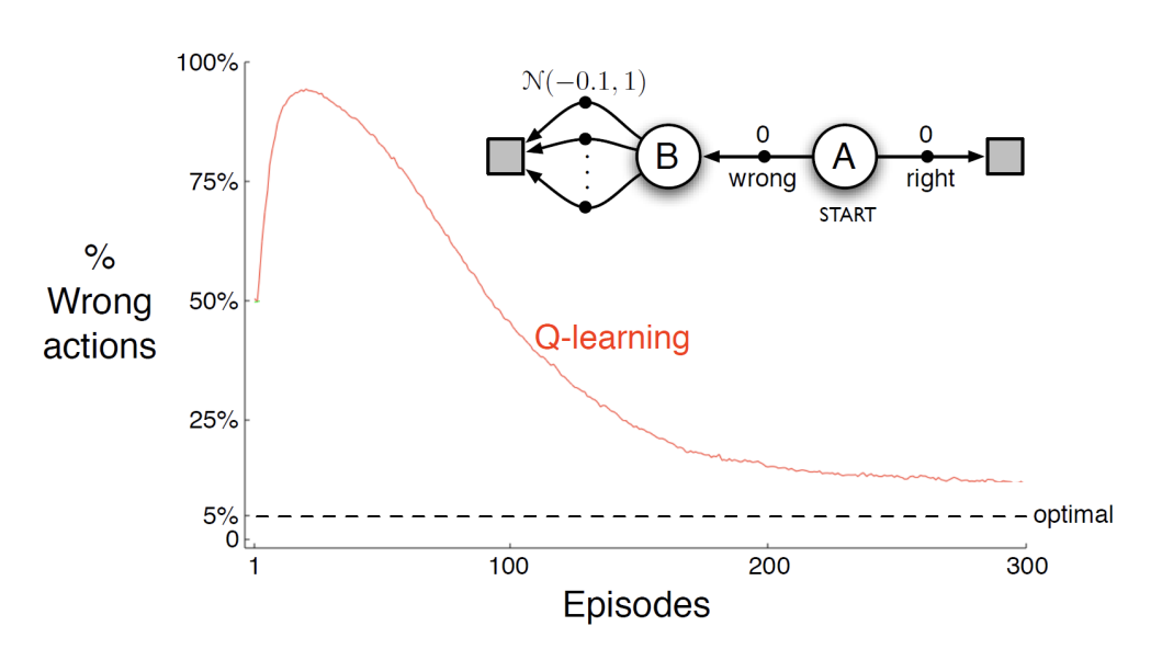
False signals from \mathcal{N}(0.1,1), may have few positive results from random noise. (However, in the long run, it will converge to the expected negative value.)

Double Q-learning

(Hado van Hasselt 2010)

Train 2 action-value functions, Q1 and Q2

Do Q-learning on both, but

• never on the same time steps (Q1 and Q2 are indep.)
• pick Q1 or Q2 at random to be updated on each step

If updating Q1, use Q2 for the value of the next state:

Q_1(S_t,A_t) \gets Q_1(S_t,A_t) + \alpha (R_{t+1} + \gamma Q_2(S_{t+1}, \arg\max_{a'\in A} Q_1(S_{t+1},a')) - Q_1(S_t,A_t))

Action selections are (say) $\epsilon$-greedy with respect to the sum of Q1 and Q2. (unbiased estimation and same convergence as Q-learning)

Drawbacks:

• More computationally expensive (only one function is trained at a time)

Initialize Q1 and Q2
For each episode:
    Initialize state
    For each step:
        Choose $A$ from $S$ using policy derived from Q1 and Q2
        Take action $A$, observe $R$ and $S'$
        With probability $0.5$, update Q1:
            $Q1(S,A) \gets Q1(S,A) + \alpha (R + \gamma Q2(S', \arg\max_{a'\in A} Q1(S',a')) - Q1(S,A))$
        Otherwise, update Q2:
            $Q2(S,A) \gets Q2(S,A) + \alpha (R + \gamma Q1(S', \arg\max_{a'\in A} Q2(S',a')) - Q2(S,A))$
        $S \gets S'$
    End for
End for

Double DQN

(van Hasselt, Guez, Silver, 2015)

A better implementation of Double Q-learning.

• Dealing with maximization bias of Q-Learning
• Current Q-network w is used to select actions
• Older Q-network w^- is used to evaluate actions

l=\left(r+\gamma Q(s', \arg\max_{a'\in A} Q(s',a';w);w^-) - Q(s,a;w)\right)^2

Here \arg\max_{a'\in A} Q(s',a';w) is the action selected by the current Q-network w.

Q(s', \arg\max_{a'\in A} Q(s',a';w);w^-) is the action evaluation by the older Q-network w^-.

Prioritized Experience Replay

(Schaul, Quan, Antonoglou, Silver, ICLR 2016)

Weight experience according to "surprise" (or error)

• Store experience in priority queue according to DQN error

  
  \left|r+\gamma \arg\max_{a'\in A} Q(s',a',w^-)-Q(s,a,w)\right|
  

• Stochastic Prioritization

  
  P(i)=\frac{p_i^\alpha}{\sum_k p_k^\alpha}
  

  • p_i is proportional to the DQN error

• \alpha determines how much prioritization is used, with \alpha = 0 corresponding to the uniform case.

Dueling Q networks

(Wang et.al., ICML, 2016)

• Split Q-network into two channels

  • Action-independent value function V(s; w): measures how good is the state s

  • Action-dependent advantage function A(s, a; w): measure how much better is action a than the average action in state s

    
    Q(s,a; w) = V(s; w) + A(s, a; w)
    

• Advantage function is defined as:

  
  A^\pi(s, a) = Q^\pi(s, a) - V^\pi(s)
  

The value stream learns to pay attention to the road

The advantage stream: pay attention only when there are cars immediately in front, so as to avoid collisions

Multistep returns

Truncated n-step return from a state s_t

R^{n}_t = \sum_{i=0}^{n-1} \gamma^{(k)}_t R_{t+k+1}

Multistep Q-learning update rule:

I=\left(R^{n}_t + \gamma^{(n)}_t \max_{a'\in A} Q(s_{t+n},a';w)-Q(s,a,w)\right)^2

Singlestep Q-learning update rule:

I=\left(r+\gamma \max_{a'\in A} Q(s',a';w)-Q(s,a,w)\right)^2

Distributed DQN

• Separating Learning from Acting
• Distributing hundreds of actors over CPUs
• Advantages: better harnessing computation, local priority evaluation, better exploration

Distributed DQN with Recurrent Experience Replay (R2D2)

Providing an LSTM layer after the convolutional stack

• To deal with partial observability

Other tricks:

• prioritized distributed replay
• n-step double Q-learning (with n = 5)
• generating experience by a large number of actors (typically 256)
• learning from batches of replayed experience by a single learner

Agent 57

link to paper