512 lines
19 KiB
Markdown
512 lines
19 KiB
Markdown
# CSE5519 Advances in Computer Vision (Topic E: 2021 and before: Deep Learning for Geometric Computer Vision)
|
|
|
|
> [!NOTE]
|
|
>
|
|
> This topic is presented by Me. and will be the most detailed one for this course, perhaps.
|
|
|
|
## Data set of the scene: KITTI
|
|
|
|
[link to the website](http://www.cvlibs.net/datasets/kitti/)
|
|
|
|
## PoseNet
|
|
|
|
A Convolutional Network for Real-Time 6-DOF Camera Relocalization (ICCV 2015)
|
|
|
|
Problem solving:
|
|
|
|
Camera Pose: Camera position and orientation.
|
|
|
|
[link to the paper](https://arxiv.org/pdf/1505.07427)
|
|
|
|
Convolutional neural network (convnet) we train to estimate camera pose directly
|
|
from a monocular image, $I$. Our network outputs a pose
|
|
vector $p$, given by a 3D camera position $x$ and orientation
|
|
represented by quaternion q:
|
|
|
|
$$
|
|
p = [x, q]
|
|
$$
|
|
|
|
$q$ is a quaternion, $x$ is a 3D camera position.
|
|
|
|
Arbitrary 4D values are easily mapped to legitimate rotations by normalizing them to unit length.
|
|
|
|
### Regression function
|
|
|
|
Use Stochastic Gradient Descent (SGD) to optimize the network parameters.
|
|
|
|
$$
|
|
loss(I)=\|\hat{x}-x\|_2+\beta\left\|\hat{q}-\frac{q}{\|q\|}\right\|_2
|
|
$$
|
|
|
|
$\hat{x}$ is the estimated camera position, $x$ is the ground truth camera position, $\hat{q}$ is the estimated camera orientation, $q$ is the ground truth camera orientation.
|
|
|
|
$\beta$ is a hyperparameter that scale the loss of the camera orientation so that the network can balance on estimating the camera position and orientation approximately the same weight.
|
|
|
|
### Network architecture
|
|
|
|
Based on GoogLeNet (SOTA in 2014), but with a few changes:
|
|
|
|
- Replace all three softmax classifiers with affine regressors.
|
|
- Insert another fully connected layer before final regressor of feature size 2048
|
|
- At test time, normalize the quaternion to unit length.
|
|
|
|
<details>
|
|
<summary>Architecture</summary>
|
|
|
|
```python
|
|
from network import Network
|
|
|
|
class GoogLeNet(Network):
|
|
def setup(self):
|
|
(self.feed('data')
|
|
.conv(7, 7, 64, 2, 2, name='conv1')
|
|
.max_pool(3, 3, 2, 2, name='pool1')
|
|
.lrn(2, 2e-05, 0.75, name='norm1')
|
|
.conv(1, 1, 64, 1, 1, name='reduction2')
|
|
.conv(3, 3, 192, 1, 1, name='conv2')
|
|
.lrn(2, 2e-05, 0.75, name='norm2')
|
|
.max_pool(3, 3, 2, 2, name='pool2')
|
|
.conv(1, 1, 96, 1, 1, name='icp1_reduction1')
|
|
.conv(3, 3, 128, 1, 1, name='icp1_out1'))
|
|
|
|
(self.feed('pool2')
|
|
.conv(1, 1, 16, 1, 1, name='icp1_reduction2')
|
|
.conv(5, 5, 32, 1, 1, name='icp1_out2'))
|
|
|
|
(self.feed('pool2')
|
|
.max_pool(3, 3, 1, 1, name='icp1_pool')
|
|
.conv(1, 1, 32, 1, 1, name='icp1_out3'))
|
|
|
|
(self.feed('pool2')
|
|
.conv(1, 1, 64, 1, 1, name='icp1_out0'))
|
|
|
|
(self.feed('icp1_out0',
|
|
'icp1_out1',
|
|
'icp1_out2',
|
|
'icp1_out3')
|
|
.concat(3, name='icp2_in')
|
|
.conv(1, 1, 128, 1, 1, name='icp2_reduction1')
|
|
.conv(3, 3, 192, 1, 1, name='icp2_out1'))
|
|
|
|
(self.feed('icp2_in')
|
|
.conv(1, 1, 32, 1, 1, name='icp2_reduction2')
|
|
.conv(5, 5, 96, 1, 1, name='icp2_out2'))
|
|
|
|
(self.feed('icp2_in')
|
|
.max_pool(3, 3, 1, 1, name='icp2_pool')
|
|
.conv(1, 1, 64, 1, 1, name='icp2_out3'))
|
|
|
|
(self.feed('icp2_in')
|
|
.conv(1, 1, 128, 1, 1, name='icp2_out0'))
|
|
|
|
(self.feed('icp2_out0',
|
|
'icp2_out1',
|
|
'icp2_out2',
|
|
'icp2_out3')
|
|
.concat(3, name='icp2_out')
|
|
.max_pool(3, 3, 2, 2, name='icp3_in')
|
|
.conv(1, 1, 96, 1, 1, name='icp3_reduction1')
|
|
.conv(3, 3, 208, 1, 1, name='icp3_out1'))
|
|
|
|
(self.feed('icp3_in')
|
|
.conv(1, 1, 16, 1, 1, name='icp3_reduction2')
|
|
.conv(5, 5, 48, 1, 1, name='icp3_out2'))
|
|
|
|
(self.feed('icp3_in')
|
|
.max_pool(3, 3, 1, 1, name='icp3_pool')
|
|
.conv(1, 1, 64, 1, 1, name='icp3_out3'))
|
|
|
|
(self.feed('icp3_in')
|
|
.conv(1, 1, 192, 1, 1, name='icp3_out0'))
|
|
|
|
(self.feed('icp3_out0',
|
|
'icp3_out1',
|
|
'icp3_out2',
|
|
'icp3_out3')
|
|
.concat(3, name='icp3_out')
|
|
.avg_pool(5, 5, 3, 3, padding='VALID', name='cls1_pool')
|
|
.conv(1, 1, 128, 1, 1, name='cls1_reduction_pose')
|
|
.fc(1024, name='cls1_fc1_pose')
|
|
.fc(3, relu=False, name='cls1_fc_pose_xyz'))
|
|
|
|
(self.feed('cls1_fc1_pose')
|
|
.fc(4, relu=False, name='cls1_fc_pose_wpqr'))
|
|
|
|
(self.feed('icp3_out')
|
|
.conv(1, 1, 112, 1, 1, name='icp4_reduction1')
|
|
.conv(3, 3, 224, 1, 1, name='icp4_out1'))
|
|
|
|
(self.feed('icp3_out')
|
|
.conv(1, 1, 24, 1, 1, name='icp4_reduction2')
|
|
.conv(5, 5, 64, 1, 1, name='icp4_out2'))
|
|
|
|
(self.feed('icp3_out')
|
|
.max_pool(3, 3, 1, 1, name='icp4_pool')
|
|
.conv(1, 1, 64, 1, 1, name='icp4_out3'))
|
|
|
|
(self.feed('icp3_out')
|
|
.conv(1, 1, 160, 1, 1, name='icp4_out0'))
|
|
|
|
(self.feed('icp4_out0',
|
|
'icp4_out1',
|
|
'icp4_out2',
|
|
'icp4_out3')
|
|
.concat(3, name='icp4_out')
|
|
.conv(1, 1, 128, 1, 1, name='icp5_reduction1')
|
|
.conv(3, 3, 256, 1, 1, name='icp5_out1'))
|
|
|
|
(self.feed('icp4_out')
|
|
.conv(1, 1, 24, 1, 1, name='icp5_reduction2')
|
|
.conv(5, 5, 64, 1, 1, name='icp5_out2'))
|
|
|
|
(self.feed('icp4_out')
|
|
.max_pool(3, 3, 1, 1, name='icp5_pool')
|
|
.conv(1, 1, 64, 1, 1, name='icp5_out3'))
|
|
|
|
(self.feed('icp4_out')
|
|
.conv(1, 1, 128, 1, 1, name='icp5_out0'))
|
|
|
|
(self.feed('icp5_out0',
|
|
'icp5_out1',
|
|
'icp5_out2',
|
|
'icp5_out3')
|
|
.concat(3, name='icp5_out')
|
|
.conv(1, 1, 144, 1, 1, name='icp6_reduction1')
|
|
.conv(3, 3, 288, 1, 1, name='icp6_out1'))
|
|
|
|
(self.feed('icp5_out')
|
|
.conv(1, 1, 32, 1, 1, name='icp6_reduction2')
|
|
.conv(5, 5, 64, 1, 1, name='icp6_out2'))
|
|
|
|
(self.feed('icp5_out')
|
|
.max_pool(3, 3, 1, 1, name='icp6_pool')
|
|
.conv(1, 1, 64, 1, 1, name='icp6_out3'))
|
|
|
|
(self.feed('icp5_out')
|
|
.conv(1, 1, 112, 1, 1, name='icp6_out0'))
|
|
|
|
(self.feed('icp6_out0',
|
|
'icp6_out1',
|
|
'icp6_out2',
|
|
'icp6_out3')
|
|
.concat(3, name='icp6_out')
|
|
.avg_pool(5, 5, 3, 3, padding='VALID', name='cls2_pool')
|
|
.conv(1, 1, 128, 1, 1, name='cls2_reduction_pose')
|
|
.fc(1024, name='cls2_fc1')
|
|
.fc(3, relu=False, name='cls2_fc_pose_xyz'))
|
|
|
|
(self.feed('cls2_fc1')
|
|
.fc(4, relu=False, name='cls2_fc_pose_wpqr'))
|
|
|
|
(self.feed('icp6_out')
|
|
.conv(1, 1, 160, 1, 1, name='icp7_reduction1')
|
|
.conv(3, 3, 320, 1, 1, name='icp7_out1'))
|
|
|
|
(self.feed('icp6_out')
|
|
.conv(1, 1, 32, 1, 1, name='icp7_reduction2')
|
|
.conv(5, 5, 128, 1, 1, name='icp7_out2'))
|
|
|
|
(self.feed('icp6_out')
|
|
.max_pool(3, 3, 1, 1, name='icp7_pool')
|
|
.conv(1, 1, 128, 1, 1, name='icp7_out3'))
|
|
|
|
(self.feed('icp6_out')
|
|
.conv(1, 1, 256, 1, 1, name='icp7_out0'))
|
|
|
|
(self.feed('icp7_out0',
|
|
'icp7_out1',
|
|
'icp7_out2',
|
|
'icp7_out3')
|
|
.concat(3, name='icp7_out')
|
|
.max_pool(3, 3, 2, 2, name='icp8_in')
|
|
.conv(1, 1, 160, 1, 1, name='icp8_reduction1')
|
|
.conv(3, 3, 320, 1, 1, name='icp8_out1'))
|
|
|
|
(self.feed('icp8_in')
|
|
.conv(1, 1, 32, 1, 1, name='icp8_reduction2')
|
|
.conv(5, 5, 128, 1, 1, name='icp8_out2'))
|
|
|
|
(self.feed('icp8_in')
|
|
.max_pool(3, 3, 1, 1, name='icp8_pool')
|
|
.conv(1, 1, 128, 1, 1, name='icp8_out3'))
|
|
|
|
(self.feed('icp8_in')
|
|
.conv(1, 1, 256, 1, 1, name='icp8_out0'))
|
|
|
|
(self.feed('icp8_out0',
|
|
'icp8_out1',
|
|
'icp8_out2',
|
|
'icp8_out3')
|
|
.concat(3, name='icp8_out')
|
|
.conv(1, 1, 192, 1, 1, name='icp9_reduction1')
|
|
.conv(3, 3, 384, 1, 1, name='icp9_out1'))
|
|
|
|
(self.feed('icp8_out')
|
|
.conv(1, 1, 48, 1, 1, name='icp9_reduction2')
|
|
.conv(5, 5, 128, 1, 1, name='icp9_out2'))
|
|
|
|
(self.feed('icp8_out')
|
|
.max_pool(3, 3, 1, 1, name='icp9_pool')
|
|
.conv(1, 1, 128, 1, 1, name='icp9_out3'))
|
|
|
|
(self.feed('icp8_out')
|
|
.conv(1, 1, 384, 1, 1, name='icp9_out0'))
|
|
|
|
(self.feed('icp9_out0',
|
|
'icp9_out1',
|
|
'icp9_out2',
|
|
'icp9_out3')
|
|
.concat(3, name='icp9_out')
|
|
.avg_pool(7, 7, 1, 1, padding='VALID', name='cls3_pool')
|
|
.fc(2048, name='cls3_fc1_pose')
|
|
.fc(3, relu=False, name='cls3_fc_pose_xyz'))
|
|
|
|
(self.feed('cls3_fc1_pose')
|
|
.fc(4, relu=False, name='cls3_fc_pose_wpqr'))
|
|
```
|
|
|
|
</details>
|
|
|
|
## Unsupervised Learning of Depth and Ego-Motion From Video
|
|
|
|
(CVPR 2017)
|
|
|
|
[link to the paper](https://openaccess.thecvf.com/content_cvpr_2017/papers/Zhou_Unsupervised_Learning_of_CVPR_2017_paper.pdf)
|
|
|
|
This is a method that estimates both depth and camera pose motion from a single video using CNN.
|
|
|
|
Jointly training a single-view depth CNN and a camera pose estimation CNN form unlabelled monocular video sequences.
|
|
|
|
### Assumptions for PoseNet & DepthNet
|
|
|
|
1. The scene is static and the only motion is the camera motion.
|
|
2. There is no occlusion/disocclusion between the target view and the source view.
|
|
3. The surface is Lambertian.
|
|
|
|
|
|
|
|
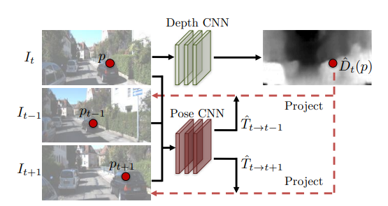
Let $I_{t-1}, I_{t}, I_{t+1}$ be three consecutive frames in the video.
|
|
|
|
First, we use the DepthNet to estimate the depth of $I_t$ to obtain $\hat{D}_t$. We use the PoseNet to estimate the camera pose motion between $I_{t-1}$ and $I_{t+1}$ to obtain two transition vector $\hat{T}_{t\to t-1}$ and $\hat{T}_{t\to t+1}$.
|
|
|
|
Then use the information we have from $\hat{D}_t$ and $\hat{T}_{t\to t-1}, \hat{T}_{t\to t+1}$ with frame $I_{t-1}$ and $I_{t+1}$ to synthesize the image $\hat{I}_s$ from $I_{t-1}$ and $I_{t+1}$.
|
|
|
|
Note that $\hat{I}_s$ is the synthesized prediction for $I_t$.
|
|
|
|
### Loss function for PoseNet & DepthNet
|
|
|
|
Notice that in the training process, we can generate the supervision for PoseNet & DepthNet by using **view synthesis as supervision**.
|
|
|
|
#### View synthesis as supervision
|
|
|
|
Let $\mathcal{I}=\{I_1,I_2,I_3,\cdots,I_n\}$ be the video sequence. Note that $I_t(p)$ is the pixel value of $I_t$ at point $p$.
|
|
|
|
The loss function generated by view synthesis is:
|
|
|
|
$$
|
|
\mathcal{L}_{vs}=\sum_{I_s\in\mathcal{I}}\sum_{p\in I_s}\left|I_t(p)-\hat{I}_s(p)\right|
|
|
$$
|
|
|
|
#### Differentiable depth image-based rendering
|
|
|
|
Assume that the transition and rotation between the frames are smooth and differentiable.
|
|
|
|
Let $p_t$ denote the pixel coordinates of $I_t$ at time $t$. Let $K$ denote the camera intrinsic matrix. We can always obtain $p_t$'s projected coordinates to our source view $p_s$ by the formula:
|
|
|
|
$$
|
|
p_s\sim K\hat{T}_{t\to s}\hat{D}_t(p_t)K^{-1}p_t
|
|
$$
|
|
|
|
Then we use spacial transformer network to sample continuous pixel coordinates.
|
|
|
|
### Compensation for PoseNet & DepthNet
|
|
|
|
Since it's inevitable that there are some moving objects or occlusions between the target view and the source view, in pose net we also train a few additional layers to estimate our confidence (explainability mask) of the camera motion.
|
|
|
|
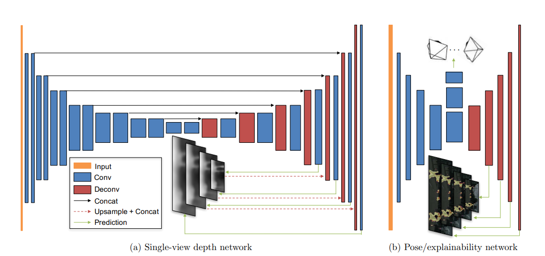
### Architecture for PoseNet & DepthNet
|
|
|
|
|
|
|
|
## Unsupervised Monocular Depth Estimation with Left-Right Consistency
|
|
|
|
(CVPR 2017)
|
|
|
|
[link to the paper](https://arxiv.org/pdf/1609.03677)
|
|
|
|
This is a method that use pair of images as Left and Right eye to estimate depth. Increased consistency by flipping the right-left relation.
|
|
|
|
**Intuition:** Given a calibarated pair of binocular cameras, if we can learn a function that is able to reconstruct one image from the other, then we have learned something about the depth of the scene.
|
|
|
|
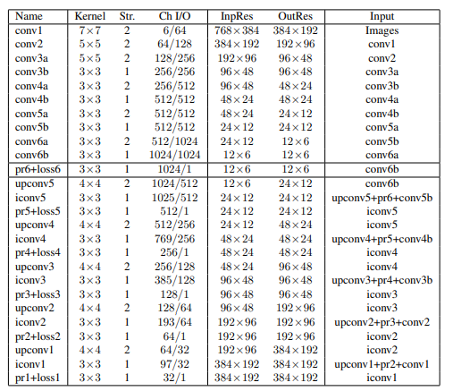
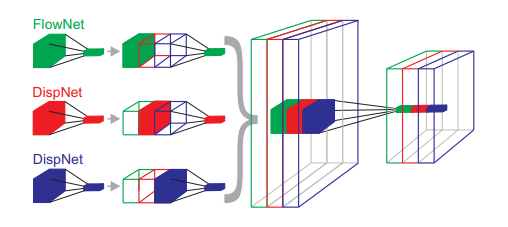
### DispNet and Scene flow
|
|
|
|
|
|
|
|
[link to the paper](https://arxiv.org/pdf/1512.02134)
|
|
|
|
#### Scene flow
|
|
|
|
Scene flow is the underlying 3D motion field that can be computed from stereo videos or RGBD videos.
|
|
|
|
Note, these 3D quantities can be computed only in the case of known camera intrinsics (i.e., $K$ matrix) and extrinsics (i.e., camera pose, translation, etc.).
|
|
|
|
Scene flow can be reconstructed only for surface points that are visible in both the left and the right frame.
|
|
|
|
Especially in the context of convolutional networks, it is particularly interesting to estimate also depth and motion in partially occluded areas
|
|
|
|
#### Disparity
|
|
|
|
Disparity is the difference in the x-coordinates of the same point in the left and right images.
|
|
|
|
|
|
|
|
If there is time difference between the "left" and "right" images, by the difference between the disparity, we can estimate the scene flow, that is, non-rigid motion of the scene.
|
|
|
|
Object that have the same disparity in both images is "moving along with the camera".
|
|
|
|
Object that is moving away, or moving toward the camera, will have higher disparity.
|
|
|
|
### Assumptions for Left-right consistency Network
|
|
|
|
1. Lambertian surface.
|
|
2. No occlusion/disocclusion between the left and right image (for computing scene flow).
|
|
|
|
### Loss functions for Left-right consistency Network
|
|
|
|
$$
|
|
\mathcal{L}=\alpha_{ap}(\mathcal{L}_{ap}^l+\mathcal{L}_{ap}^r)+\alpha_{ds}(\mathcal{L}_{ds}^l+\mathcal{L}_{ds}^r)+\alpha_{lr}(\mathcal{L}_{lr}^l+\mathcal{L}_{lr}^r)
|
|
$$
|
|
|
|
The loss function consists of three parts:
|
|
|
|
Let $N$ denote the number of pixels in the image.
|
|
|
|
#### Appearance matching loss
|
|
|
|
Let $I^l$ denote the left image, $I^r$ denote the right image, $\hat{L}^l$ denote the left image reconstructed from the right image.
|
|
|
|
$\hat{I}^l$ denote the left image reconstructed from the right image with the predicted disparity map $d^l$.
|
|
|
|
The appearance matching loss for left image is:
|
|
|
|
$$
|
|
\mathcal{L}_{ap}^l=\frac{1}{N}\sum_{p\in I^l}\alpha \frac{1-\operatorname{SSIM}(I^l(p),\hat{I}^l(p))}{2}+(1-\alpha)\left\|I^l(p)-\hat{I}^l(p)\right\|
|
|
$$
|
|
|
|
Here $\operatorname{SSIM}$ is the structural similarity index.
|
|
|
|
[link to the paper: structure similarity index](https://ieeexplore.ieee.org/stamp/stamp.jsp?tp=&arnumber=1284395)
|
|
|
|
$\alpha$ is a hyperparameter that balances the importance of the structural similarity and the pixel-wise difference. In this paper, $\alpha=0.85$.
|
|
|
|
#### Disparity Smoothness Loss
|
|
|
|
Let $\partial d$ denote the disparity gradient. $\partial_x d^l_p$ and $\partial_y d^l_p$ are the disparity gradient in the x and y directions respectively on the left image of pixel $p$.
|
|
|
|
The disparity smoothness loss is:
|
|
|
|
$$
|
|
\mathcal{L}_{ds}^l=\frac{1}{N}\sum_{p\in I^l}\left|\partial_x d^l_p\right|e^{-\left|\partial_x d^l_p\right|}+\left|\partial_y d^l_p\right|e^{-\left|\partial_y d^l_p\right|}
|
|
$$
|
|
|
|
#### Left-right disparity consistency loss
|
|
|
|
Our network produces two disparity maps, $d^l$ and $d^r$. We can use the left-right consistency loss to enforce the consistency between the two disparity maps.
|
|
|
|
$$
|
|
\mathcal{L}_{lr}^l=\frac{1}{N}\sum_{p\in I^l}\left|d^l_p-d^r_{p+d^l_p}\right|
|
|
$$
|
|
|
|
### Architecture of Left-right consistency Network
|
|
|
|

|
|
|
|
## GeoNet
|
|
|
|
Unsupervised Learning of Dense Depth, Optical Flow and Camera Pose (CVPR 2018)
|
|
|
|
Problem solving:
|
|
|
|
Depth Estimation from single monocular image.
|
|
|
|
[link to the paper](https://openaccess.thecvf.com/content_cvpr_2018/papers/Yin_GeoNet_Unsupervised_Learning_CVPR_2018_paper.pdf)
|
|
|
|
[link to the repository](https://github.com/yzcjtr/GeoNet)
|
|
|
|
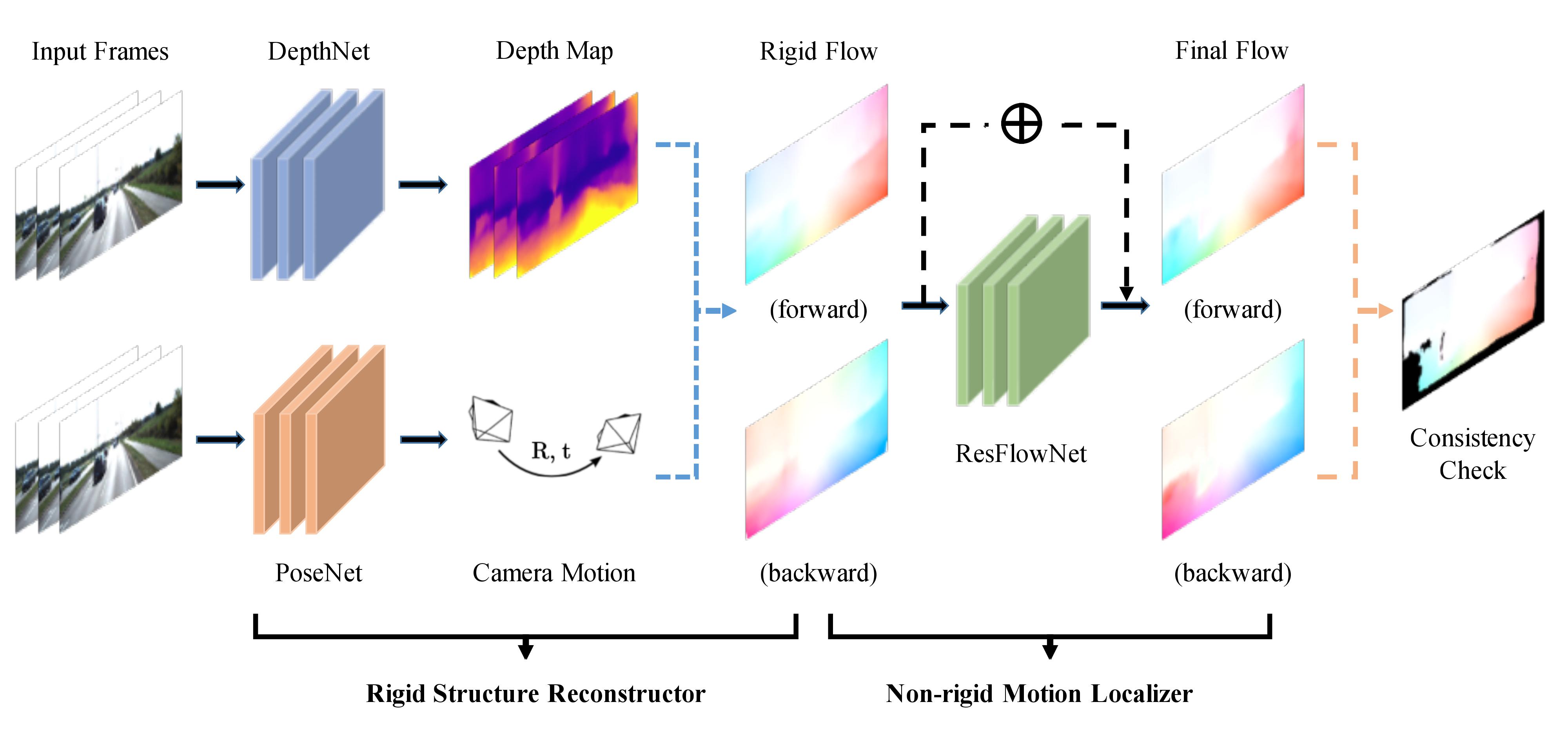
### Architecture for GeoNet
|
|
|
|
|
|
|
|
### Rigid structure constructor
|
|
|
|
Combines the DepthNet and PoseNet to estimate the depth and camera pose motion from [Unsupervised Learning of Depth and Ego-Motion From Video](#unsupervised-learning-of-depth-and-ego-motion-from-video).
|
|
|
|
We denote the output of the Rigid structure constructor from frame $t$ to $s$ as $f^{rig}_{t\to s}$. The function output is a 2D vector showing the shift of the pixel coordinates.
|
|
|
|
Recall from previous paper,
|
|
|
|
$$
|
|
\begin{aligned}
|
|
p_t+f^{rig}_{t\to s}(p_t)&=KT_{t\to s}D_t(p_t)K^{-1}p_t\\
|
|
f^{rig}_{t\to s}(p_t)&=K(T_{t\to s}D_t(p_t)+I)K^{-1}p_t-p_t
|
|
\end{aligned}
|
|
$$
|
|
|
|
### Non-rigid motion localizer
|
|
|
|
Use [Left-right consistency](#unsupervised-monocular-depth-estimation-with-left-right-consistency) to estimate the non-rigid motion by training the ResFlowNet.
|
|
|
|
We denote the output of the Non-rigid motion localizer from frame $t$ to $s$ as $f^{res}_{t\to s}$. SO the final full flow prediction is $f^{full}_{t\to s}=f^{res}_{t\to s}+f^{rig}_{t\to s}$.
|
|
|
|
Let $\hat{I}^{rig}_s$ denote the inverse wrapped image from frame $s$ to $t$. Note that $\hat{I}^{rig}_s$ is the prediction of $I_t$ from $I_s$, using the rigid structure constructor.
|
|
|
|
Recall from previous paper, we rename the $\mathcal{L}_{ap}^l$ to $\mathcal{L}_{rw}$.
|
|
|
|
$$
|
|
\mathcal{L}_{rw}=\frac{1}{N}\sum_{p\in I^l}\alpha \frac{1-\operatorname{SSIM}(I^l(p),\hat{I}^{rig}_s(p))}{2}+(1-\alpha)\left\|I^l(p)-\hat{I}^{rig}_s(p)\right\|_1\tag{1}
|
|
$$
|
|
|
|
Then we use $\mathcal{L}_{ds}$ to enforce the smoothness of the disparity map.
|
|
|
|
$$
|
|
\mathcal{L}_{ds}=\sum_{p\in I^l}\left|\partial_x d^l_p\right|e^{-\left|\partial_x d^l_p\right|}+\left|\partial_y d^l_p\right|e^{-\left|\partial_y d^l_p\right|}=\sum_{p_t}|\nabla D(p_t)|\cdot \left(e^{-|\nabla I(p_t)|}\right)^\top\tag{2}
|
|
$$
|
|
|
|
Replacing $\hat{I}^{rig}_s$ with $\hat{I}^{full}_s$, in (1) and (2), we get the $\mathcal{L}_{fw}$ and $\mathcal{L}_{fs}$ for the non-rigid motion localizer.
|
|
|
|
### Geometric consistency enforcement
|
|
|
|
Finally, we use an additional geometric consistency enforcement to handle non-Lambertian surfaces (e.g., metal, plastic, etc.).
|
|
|
|
This is done by additional term in the loss function.
|
|
|
|
Let $\Delta f^{full}_{t\to s}(p_t)=f^{full}_{t\to s}(p_t)-f^{full}_{s\to t}(p_t)$.
|
|
|
|
Let $\delta(p_t)$ denote the function belows for arbitrary $\alpha,\beta>0$:
|
|
|
|
$$
|
|
\delta(p_t)=\begin{cases}
|
|
1 & \text{if }\|\Delta f^{full}_{t\to s}(p_t)\|_2<\max\{\alpha,\beta\|f^{full}_{t\to s}(p_t)\|_1\} \\
|
|
0 & \text{otherwise}
|
|
\end{cases}
|
|
$$
|
|
|
|
The geometric consistency enforcement loss is:
|
|
|
|
$$
|
|
\mathcal{L}_{gc}=\sum_{p_t}\delta(p_t)\|\Delta f^{full}_{t\to s}(p_t)\|_2
|
|
$$
|
|
|
|
### Loss function for GeoNet
|
|
|
|
Let $l$ be the set of pyramid image scales. $\langle t,s\rangle$ denote the set of all pairs of frames in the video and their inverse pairs, $t\neq s$.
|
|
|
|
$$
|
|
\mathcal{L}=\sum_{l}\sum_{\langle t,s\rangle}\mathcal{L}_{rw}+\lambda_{ds}\mathcal{L}_{ds}+\lambda_{fw}\mathcal{L}_{fw}+\lambda_{fs}\mathcal{L}_{fs}+\lambda_{gc}\mathcal{L}_{gc}
|
|
$$
|
|
|
|
$\lambda_{ds},\lambda_{fw},\lambda_{fs},\lambda_{gc}$ are hyperparameters that balance the importance of the different losses.
|
|
|
|
### Results for monocular depth estimation
|
|
|
|
 |