203 lines
8.3 KiB
Markdown
203 lines
8.3 KiB
Markdown
# Math401 Topic 5: Introducing dynamics: classical and non-commutative
|
|
|
|
## Section 1: Dynamics in classical probability
|
|
|
|
### Basic definitions
|
|
|
|
#### Definition of orbit
|
|
|
|
Let $T:\Omega\to\Omega$ be a map (may not be invertible) generating a dynamical system on $\Omega$. Given $\omega\in \Omega$, the (forward) orbit of $\omega$ is the set $\mathscr{O}(\omega)=\{T^n(\omega)\}_{n\in\mathbb{Z}}$.
|
|
|
|
The theory of dynamics is the study of properties of orbits.
|
|
|
|
#### Definition of measure-preserving map
|
|
|
|
Let $P$ be a probability measure on a $\sigma$-algebra $\mathscr{F}$ of subsets of $\Omega$. (that is, $P:\mathscr{F}\to$ anything) A measurable transformation $T:\Omega\to\Omega$ is said to be measure-preserving if for all random variables $\psi:\Omega\to\mathbb{R}$, we have $\mathbb{E}(\psi\circ T)=\mathbb{E}(\psi)$, that is:
|
|
|
|
$$
|
|
\int_\Omega (\psi\circ T)(\omega)dP(\omega)=\int_\Omega \psi(\omega)dP(\omega)
|
|
$$
|
|
|
|
Example:
|
|
|
|
The doubling map $T:\Omega\to\Omega$ is defined as $T(x)=2x\mod 1$, is a Lebesgue measure preserving map on $\Omega=[0,1]$.
|
|
|
|
#### Definition of isometry
|
|
|
|
The composition operator $\psi\mapsto U\psi=\psi\circ T$, where $T$ is a measure preserving map defined on $\mathscr{H}=L^2(\Omega,\mathscr{F},P)$ is isometry of $\mathscr{H}$ if $\langle U\psi,U\phi\rangle=\langle\psi,\phi\rangle$ for all $\psi,\phi\in\mathscr{H}$.
|
|
|
|
#### Definition of unitary
|
|
|
|
The composition operator $\psi\mapsto U\psi=\psi\circ T$, where $T$ is a measure preserving map defined on $\mathscr{H}=L^2(\Omega,\mathscr{F},P)$ is unitary of $\mathscr{H}$ if $U$ is an isometry and $T$ is invertible with measurable inverse.
|
|
|
|
## Section 2: Continuous time (classical) dynamical systems
|
|
|
|
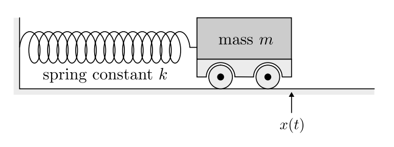
### Spring-mass system
|
|
|
|
|
|
|
|
The pure state of the system is given by the position and velocity of the mass. $(x,v)$ is a point in $\mathbb{R}^2$. $\mathbb{R}^2$ is the state space of the system. (or phase space)
|
|
|
|
The motion of the system in its state space is a closed curve.
|
|
|
|
$$
|
|
\Phi_t(x,v)=\left(\cos(\omega t)x-\frac{1}{\omega}\sin(\omega t)v, \cos(\omega t)v-\omega\sin(\omega t)x\right)
|
|
$$
|
|
|
|
Such system with closed curve is called **integrable system**. Where the doubling map produces orbits having distinct dynamical properties (**chaotic system**).
|
|
|
|
> Note, some section is intentionally ignored here. They are about in the setting of operators on Hilbert spaces, the evolution of (classical, non-dissipative e.g. linear spring-mass system) system, is implemented by a one-parameter group of unitary operators.
|
|
>
|
|
> The detailed construction is omitted here.
|
|
|
|
#### Definition of Hermitian operator
|
|
|
|
A linear operator $A$ on a Hilbert space $\mathscr{H}$ is said to be Hermitian if $\forall \psi,\phi\in$ **domain of $A$**, we have $\langle A\psi,\phi\rangle=\langle\psi,A\phi\rangle$.
|
|
|
|
It is skew-Hermitian if $\langle A\psi,\phi\rangle=-\langle\psi,A\phi\rangle$.
|
|
|
|
## Section 3: Hamiltonians and the Schrödinger equation (finite dimensional version)
|
|
|
|
the problem of solving Schrödinger equation is at its core about studying the spectral theory of the Hamiltonian operator.
|
|
|
|
### Dynamics in 2-dimensional (_2 level_) systems (qubit)
|
|
|
|
In previous sections, we know that any self-adjoint matrix has the form $x_0+\vec{x}\cdot \sigma$, where $\sigma$ is the Pauli matrices.
|
|
|
|
And $(x_0,\vec{x})\in\mathbb{R}^4$ is a point in $\mathbb{R}^4$.
|
|
|
|
The general form (time-independent) of the Hamiltonian for a 2-level system is:
|
|
|
|
$$
|
|
H=\begin{pmatrix}
|
|
x_0+x_3 & x_1-ix_2 \\
|
|
x_1+ix_2 & -x_0+x_3
|
|
\end{pmatrix}
|
|
$$
|
|
|
|
Parameterizing the curves in Bloch space generated by Hamiltonian. In physical dimension of $\vec{x}=\omega\hbar\vec{s}$, $\omega>0$. $\omega\hbar$ is the physical dimension of energy.
|
|
|
|
we have:
|
|
|
|
$$
|
|
H=\omega\hbar\begin{pmatrix}
|
|
s_3 & s_1-is_2 \\
|
|
s_1+is_2 & -s_3
|
|
\end{pmatrix}
|
|
$$
|
|
|
|
[Continue on the orbits of states in the Bloch sphere] skip for now.
|
|
|
|
## Section 4: Transition probability, probability amplitudes and the Born rule
|
|
|
|
the modulus squared of a probability amplitude is the probability of the corresponding state.
|
|
|
|
### Basic definitions in transition probability
|
|
|
|
#### Definition of probability amplitude
|
|
|
|
For a n-dimensional Hilbert space $\mathscr{H}$, the system is initially in a pure state give by the unit vector $|\psi_0\rangle\in\mathscr{H}$, thus with the density operator $\rho_0=|\psi_0\rangle\langle\psi_0|$.
|
|
|
|
Then the state at time $t_1$ is given by $|\psi_1\rangle=A|\psi_0\rangle$, where $A\in U(n)$ is a unitary operator.
|
|
|
|
Then the density operator at time $t_1$ is given by $\rho_1=|\psi_1\rangle\langle\psi_1|=A|\psi_0\rangle\langle\psi_0|A^*=A\rho_0A^*$.
|
|
|
|
The entry of $A$ are $a_{ij}=\langle i|A|j\rangle$. where $|i\rangle$ is the basis of $\mathscr{H}$.
|
|
|
|
The $a_{ij}$ are the probability amplitudes of the transition from state $|i\rangle$ to state $|j\rangle$.
|
|
|
|
#### Definition of transition probability
|
|
|
|
Given above, the transition probability from state $|i\rangle$ to state $|j\rangle$ is given by:
|
|
|
|
$$
|
|
|a_{ij}|^2
|
|
$$
|
|
|
|
#### Sum over paths
|
|
|
|
To each path of classical states, path $j\to i: i_0=j,i_1,i_2,\cdots,i_l=i$, we associates the probability amplitude of the path given by:
|
|
|
|
$$
|
|
|\text{path}(j\to i)\rangle=\langle i_0|i_1\rangle\langle i_1|i_2\rangle\cdots\langle i_{l-1}|i_l\rangle
|
|
$$
|
|
|
|
The probability of the path is given by:
|
|
|
|
$$
|
|
\operatorname{Prob}(i|j)=\left|\sum_{\text{all paths}j\to i \text{ with } l \text{ steps}}|\text{path}(j\to i)\rangle\right|^2
|
|
$$
|
|
|
|
### Measuring a qubit
|
|
|
|
#### Definition of qubit
|
|
|
|
A qubit is a 2-level quantum system.
|
|
|
|
One example of qubit is the photon polarization.
|
|
|
|
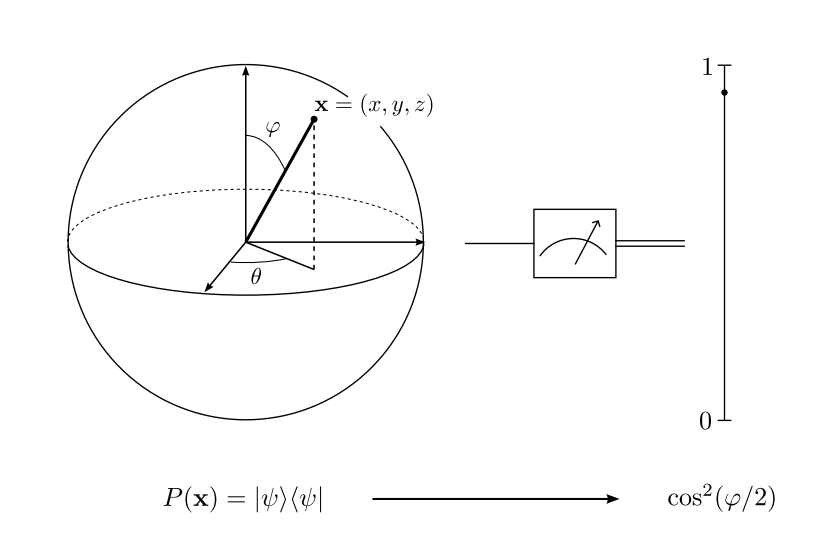
#### Measurement of a qubit
|
|
|
|
The measurement of a qubit is a map fro the space of density operators, to a point on the intervals $[0,1]$.
|
|
|
|
This gives a probability distribution on the interval $[0,1]$ in our classical probability space.
|
|
|
|
|
|
|
|
Here $p=\cos^2(\theta)\in[0,1]$. is the probability of the state being in the state $|0\rangle$.
|
|
|
|
The north pole on the Bloch sphere gives probability $1$ for the state being in the state $|0\rangle$.
|
|
|
|
The south pole on the Bloch sphere gives probability $1$ for the state being in the state $|1\rangle$.
|
|
|
|
The equator on the Bloch sphere gives probability $1/2$ for the state being in the state $|0\rangle$ or $|1\rangle$.
|
|
|
|
### Projective measurement of an $N$-qubit system
|
|
|
|
For $N$ qubits, the pure quantum state $\rho=|\psi\rangle\langle\psi|$ represented by the state vector $|\psi\rangle\in\mathscr{H}^{\otimes N}=\mathscr{H}\otimes\cdots\otimes\mathscr{H}(\mathscr{H}=\mathbb{C}^2)$.
|
|
|
|
This produces as output the random variable $X\in \{0,1\}^N$. $X=(a_1,a_2,\cdots,a_N)$, where $a_i\in \{0,1\}$.
|
|
|
|
By the Born rule,
|
|
|
|
$$
|
|
\operatorname{Prob}(X=(a_1,a_2,\cdots,a_N))=\left|\langle a_1a_2\cdots a_N|\psi\rangle\right|^2
|
|
$$
|
|
|
|
where $\langle a_1a_2\cdots a_N|\psi\rangle=\langle a_1|\otimes\langle a_2|\otimes\cdots\otimes\langle a_N|\psi\rangle$.
|
|
|
|
The input vector state $|\psi\rangle$ is a unit vector in $\mathscr{H}^{\otimes N}$.
|
|
|
|
This can be written as a tensor product of the basis vectors:
|
|
|
|
$$
|
|
|\psi\rangle=\sum_{a_1,a_2,\cdots,a_N} c_{a_1,a_2,\cdots,a_N}|a_1a_2\cdots a_N\rangle
|
|
$$
|
|
|
|
where $c_{a_1,a_2,\cdots,a_N}\in\mathbb{C}$.
|
|
|
|
The probability distribution of the post-measurement **classical random variable** $X$ can be represented as a point in the $2^N-1$ dimensional simplex of all probability distributions on the set $\{0,1\}^N$.
|
|
|
|
$$
|
|
\mathscr{P}(\{0,1\}^N)=\left\{(p_1,p_2,\cdots,p_{2^N})\in\mathbb{R}^{2^N}:p_i\geq 0,\sum_{i=1}^{2^N}p_i=1\right\}
|
|
$$
|
|
|
|

|
|
|
|
here we use the binary representation for the index $i$ in the diagram.
|
|
|
|
#### Pure versus mixed states
|
|
|
|
A pure state is a state that is represented by a unit vector in $\mathscr{H}^{\otimes N}$.
|
|
|
|
A mixed state is a state that is represented by a density operator in $\mathscr{H}^{\otimes N}$. (convex combination of pure states)
|
|
|
|
if $\rho_j=|\psi_j\rangle\langle\psi_j|$, then $\rho=\sum_{j=1}^N p_j\rho_j$ is a mixed state, where $p_j\geq 0$ and $\sum_{j=1}^N p_j=1$.
|
|
|
|
#### Projective measurement of subsystem and partial trace
|
|
|
|
This section is related to quantum random walk and we will skip it for now.
|
|
|
|
## Section 5: Quantum random walk
|
|
|
|
This part is skipped, it is an interesting topic, but it is not the focus of my research for now. |