149 lines
4.4 KiB
Markdown
149 lines
4.4 KiB
Markdown
# CSE559A Lecture 10
|
|
|
|
## Convolutional Neural Networks
|
|
|
|
### Convolutional Layer
|
|
|
|
Output feature map resolution depends on padding and stride
|
|
|
|
Padding: add zeros around the input image
|
|
|
|
Stride: the step of the convolution
|
|
|
|
Example:
|
|
|
|
1. Convolutional layer for 5x5 image with 3x3 kernel, padding 1, stride 1 (no skipping pixels)
|
|
- Input: 5x5 image
|
|
- Output: 3x3 feature map, (5-3+2*1)/1+1=5
|
|
2. Convolutional layer for 5x5 image with 3x3 kernel, padding 1, stride 2 (skipping pixels)
|
|
- Input: 5x5 image
|
|
- Output: 2x2 feature map, (5-3+2*1)/2+1=2
|
|
|
|
_Learned weights can be thought of as local templates_
|
|
|
|
```python
|
|
import torch
|
|
import torch.nn as nn
|
|
|
|
# suppose input image is HxWx3 (assume RGB image)
|
|
|
|
conv_layer = nn.Conv2d(in_channels=3, # input channel, input is HxWx3
|
|
out_channels=64, # output channel (number of filters), output is HxWx64
|
|
kernel_size=3, # kernel size
|
|
padding=1, # padding, this ensures that the output feature map has the same resolution as the input image, H_out=H_in, W_out=W_in
|
|
stride=1) # stride
|
|
```
|
|
|
|
Usually followed by a ReLU activation function
|
|
|
|
```python
|
|
conv_layer = nn.Conv2d(in_channels=3, out_channels=64, kernel_size=3, padding=1, stride=1)
|
|
relu = nn.ReLU()
|
|
```
|
|
|
|
Suppose input image is $H\times W\times K$, the output feature map is $H\times W\times L$ with kernel size $F\times F$, this takes $F^2\times K\times L\times H\times W$ parameters
|
|
|
|
Each operation $D\times (K^2C)$ matrix with $(K^2C)\times N$ matrix, assume $D$ filters and $C$ output channels.
|
|
|
|
### Variants 1x1 convolutions, depthwise convolutions
|
|
|
|
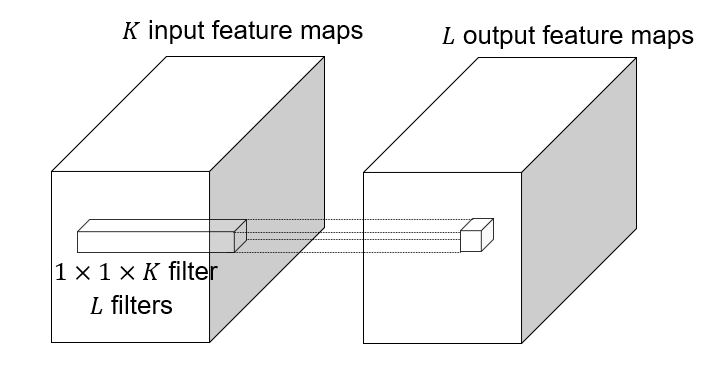
#### 1x1 convolutions
|
|
|
|
|
|
|
|
1x1 convolution: $F=1$, this layer do convolution in the pixel level, it is **pixel-wise** convolution for the feature.
|
|
|
|
Used to save computation, reduce the number of parameters.
|
|
|
|
Example: 3x3 conv layer with 256 channels at input and output.
|
|
|
|
Option 1: naive way:
|
|
|
|
```python
|
|
conv_layer = nn.Conv2d(in_channels=256, out_channels=256, kernel_size=3, padding=1, stride=1)
|
|
```
|
|
|
|
This takes $256\times 3 \times 3\times 256=524,288$ parameters.
|
|
|
|
Option 2: 1x1 convolution:
|
|
|
|
```python
|
|
conv_layer = nn.Conv2d(in_channels=256, out_channels=64, kernel_size=1, padding=0, stride=1)
|
|
conv_layer = nn.Conv2d(in_channels=64, out_channels=64, kernel_size=3, padding=1, stride=1)
|
|
conv_layer = nn.Conv2d(in_channels=64, out_channels=256, kernel_size=1, padding=0, stride=1)
|
|
```
|
|
|
|
This takes $256\times 1\times 1\times 64 + 64\times 3\times 3\times 64 + 64\times 1\times 1\times 256 = 16,384 + 36,864 + 16,384 = 69,632$ parameters.
|
|
|
|
This lose some information, but save a lot of parameters.
|
|
|
|
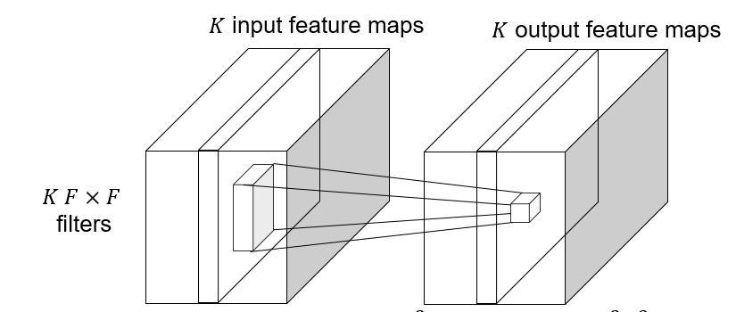
#### Depthwise convolutions
|
|
|
|
Depthwise convolution: $K\to K$ feature map, save computation, reduce the number of parameters.
|
|
|
|
|
|
|
|
#### Grouped convolutions
|
|
|
|
Self defined convolution on the feature map following the similar manner.
|
|
|
|
### Backward pass
|
|
|
|
Vector-matrix form:
|
|
|
|
$$
|
|
\frac{\partial e}{\partial x}=\frac{\partial e}{\partial z}\frac{\partial z}{\partial x}
|
|
$$
|
|
|
|
Suppose the kernel is 3x3, the feature map is $\ldots, x_{i-1}, x_i, x_{i+1}, \ldots$, and $\ldots, z_{i-1}, z_i, z_{i+1}, \ldots$ is the output feature map, then:
|
|
|
|
The convolution operation can be written as:
|
|
|
|
$$
|
|
z_i = w_1x_{i-1} + w_2x_i + w_3x_{i+1}
|
|
$$
|
|
|
|
The gradient of the kernel is:
|
|
|
|
$$
|
|
\frac{\partial e}{\partial x_i} = \sum_{j=-1}^{1}\frac{\partial e}{\partial z_i}\frac{\partial z_i}{\partial x_i} = \sum_{j=-1}^{1}\frac{\partial e}{\partial z_i}w_j
|
|
$$
|
|
|
|
### Max-pooling
|
|
|
|
Get max value in the local region.
|
|
|
|
#### Receptive field
|
|
|
|
The receptive field of a unit is the region of the input feature map whose values contribute to the response of that unit (either in the previous layer or in the initial image)
|
|
|
|
## Architecture of CNNs
|
|
|
|
### AlexNet (2012-2013)
|
|
|
|
Successor of LeNet-5, but with a few significant changes
|
|
|
|
- Max pooling, ReLU nonlinearity
|
|
- Dropout regularization
|
|
- More data and bigger model (7 hidden layers, 650K units, 60M params)
|
|
- GPU implementation (50x speedup over CPU)
|
|
- Trained on two GPUs for a week
|
|
|
|
#### Key points
|
|
|
|
Most floating point operations occur in the convolutional layers.
|
|
|
|
Most of the memory usage is in the early convolutional layers.
|
|
|
|
Nearly all parameters are in the fully-connected layers.
|
|
|
|
### VGGNet (2014)
|
|
|
|
### GoogLeNet (2014)
|
|
|
|
### ResNet (2015)
|
|
|
|
### Beyond ResNet (2016 and onward): Wide ResNet, ResNeXT, DenseNet
|
|
|
|
|