132 lines
4.2 KiB
Markdown
132 lines
4.2 KiB
Markdown
# CSE559A Lecture 15
|
||
|
||
## Continue on object detection
|
||
|
||
### Two strategies for object detection
|
||
|
||
#### R-CNN: Region proposals + CNN features
|
||
|
||

|
||
|
||
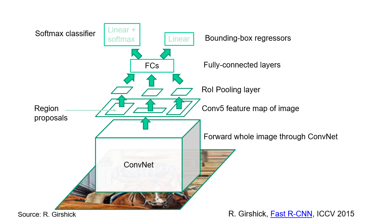
#### Fast R-CNN: CNN features + RoI pooling
|
||
|
||
|
||
|
||
Use bilinear interpolation to get the features of the proposal.
|
||
|
||
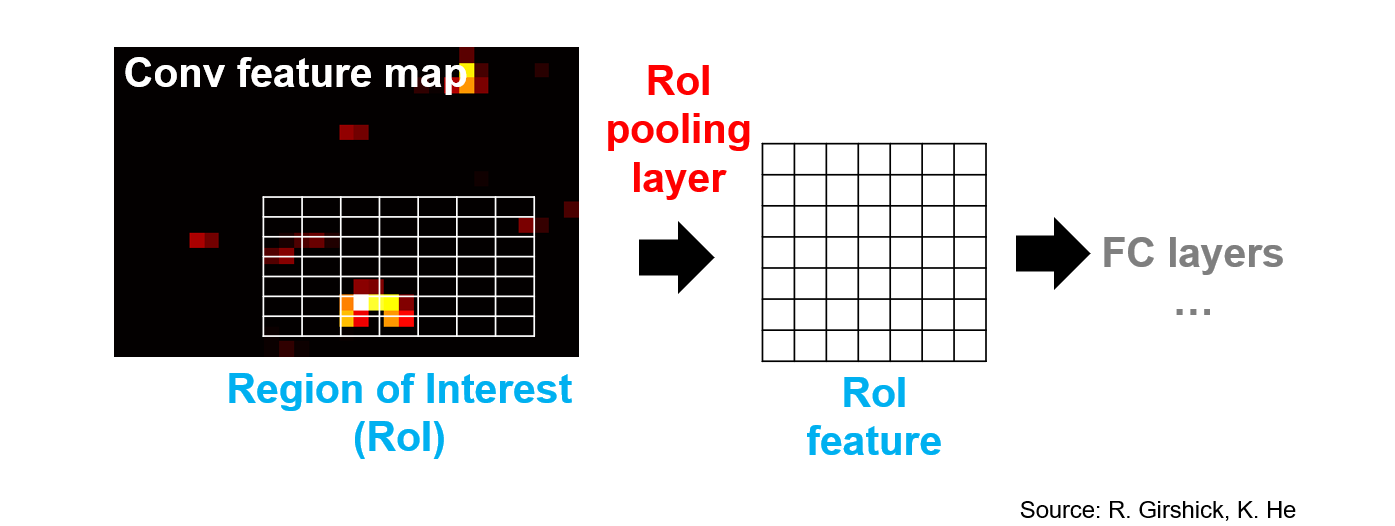
#### Region of interest pooling
|
||
|
||
|
||
|
||
Use backpropagation to get the gradient of the proposal.
|
||
|
||
### New materials
|
||
|
||
#### Faster R-CNN
|
||
|
||
Use one CNN to generate region proposals. And use another CNN to classify the proposals.
|
||
|
||
##### Region proposal network
|
||
|
||
Idea: put an "anchor box" of fixed size over each position in the feature map and try to predict whether this box is likely to contain an object.
|
||
|
||
Introduce anchor boxes at multiple scales and aspect ratios to handle a wider range of object sizes and shapes.
|
||
|
||
|
||
|
||
### Single-stage and multi-resolution detection
|
||
|
||
#### YOLO
|
||
|
||
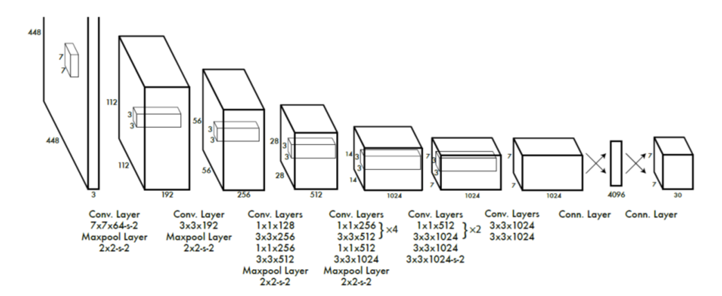
You only look once (YOLO) is a state-of-the-art, real-time object detection system.
|
||
|
||
1. Take conv feature maps at 7x7 resolution
|
||
2. Add two FC layers to predict, at each location, a score for each class and 2 bboxes with confidences
|
||
|
||
For PASCAL, output is 7×7×30 (30=20 + 2∗(4+1))
|
||
|
||
|
||
|
||
##### YOLO Network Head
|
||
|
||
```python
|
||
model.add(Conv2D(1024, (3, 3), activation='lrelu', kernel_regularizer=l2(0.0005)))
|
||
model.add(Conv2D(1024, (3, 3), activation='lrelu', kernel_regularizer=l2(0.0005)))
|
||
# use flatten layer for global reasoning
|
||
model.add(Flatten())
|
||
model.add(Dense(512))
|
||
model.add(Dense(1024))
|
||
model.add(Dropout(0.5))
|
||
model.add(Dense(7 * 7 * 30, activation='sigmoid'))
|
||
model.add(YOLO_Reshape(target_shape=(7, 7, 30)))
|
||
model.summary()
|
||
```
|
||
|
||
#### YOLO results
|
||
|
||
1. Each grid cell predicts only two boxes and can only have one class – this limits the number of nearby objects that can be predicted
|
||
2. Localization accuracy suffers compared to Fast(er) R-CNN due to coarser features, errors on small boxes
|
||
3. 7x speedup over Faster R-CNN (45-155 FPS vs. 7-18 FPS)
|
||
|
||
#### YOLOv2
|
||
|
||
1. Remove FC layer, do convolutional prediction with anchor boxes instead
|
||
2. Increase resolution of input images and conv feature maps
|
||
3. Improve accuracy using batch normalization and other tricks
|
||
|
||
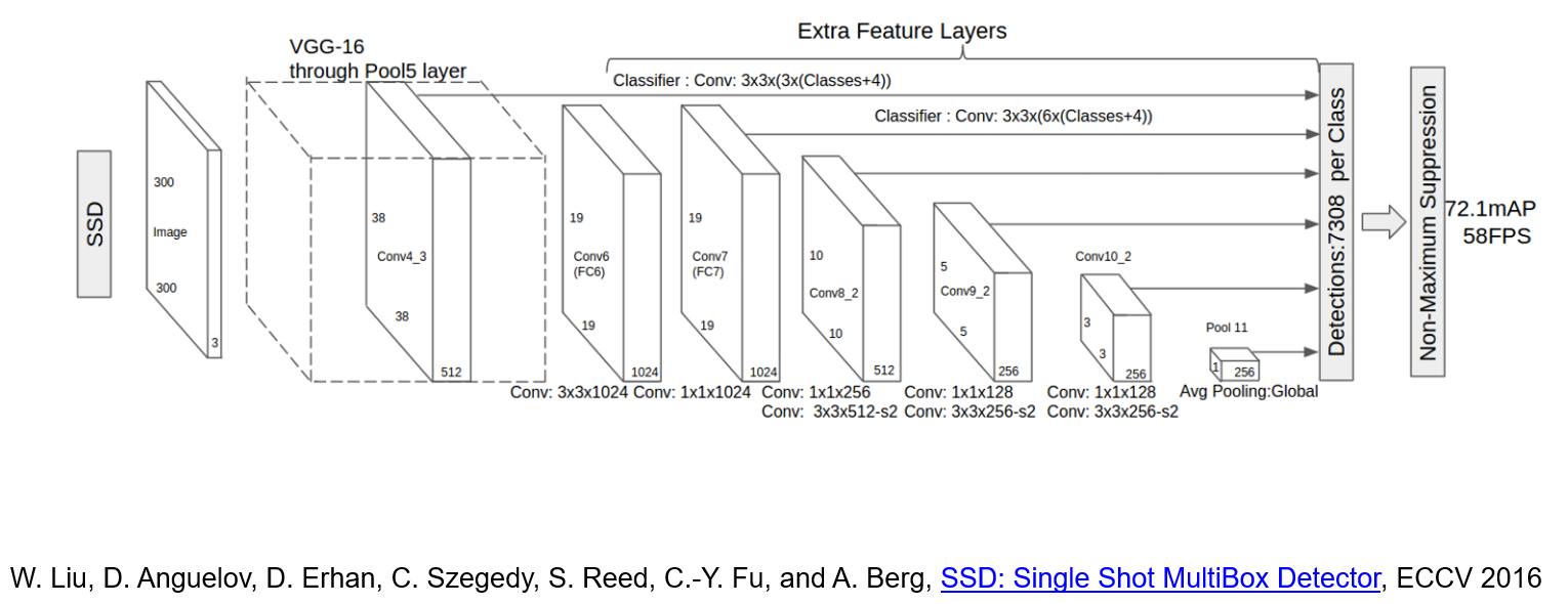
#### SSD
|
||
|
||
SSD is a multi-resolution object detection
|
||
|
||
|
||
|
||
1. Predict boxes of different size from different conv maps
|
||
2. Each level of resolution has its own predictor
|
||
|
||
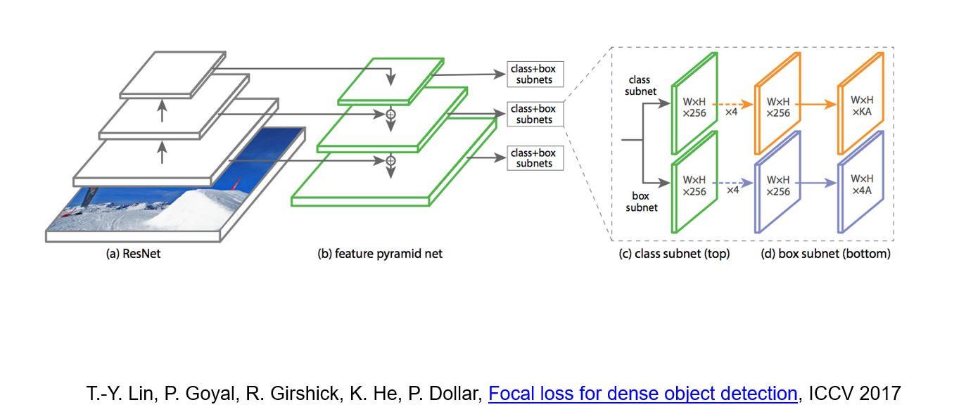
##### Feature Pyramid Network
|
||
|
||
- Improve predictive power of lower-level feature maps by adding contextual information from higher-level feature maps
|
||
- Predict different sizes of bounding boxes from different levels of the pyramid (but share parameters of predictors)
|
||
|
||
#### RetinaNet
|
||
|
||
RetinaNet combine feature pyramid network with focal loss to reduce the standard cross-entropy loss for well-classified examples.
|
||
|
||
|
||
|
||
> Cross-entropy loss:
|
||
> $$CE(p_t) = - \log(p_t)$$
|
||
|
||
The focal loss is defined as:
|
||
|
||
$$
|
||
FL(p_t) = - (1 - p_t)^{\gamma} \log(p_t)
|
||
$$
|
||
|
||
We can increase $\gamma$ to reduce the loss for well-classified examples.
|
||
|
||
#### YOLOv3
|
||
|
||
Minor refinements
|
||
|
||
### Alternative approaches
|
||
|
||
#### CornerNet
|
||
|
||
Use a pair of corners to represent the bounding box.
|
||
|
||
Use hourglass network to accumulate the information of the corners.
|
||
|
||
#### CenterNet
|
||
|
||
Use a center point to represent the bounding box.
|
||
|
||
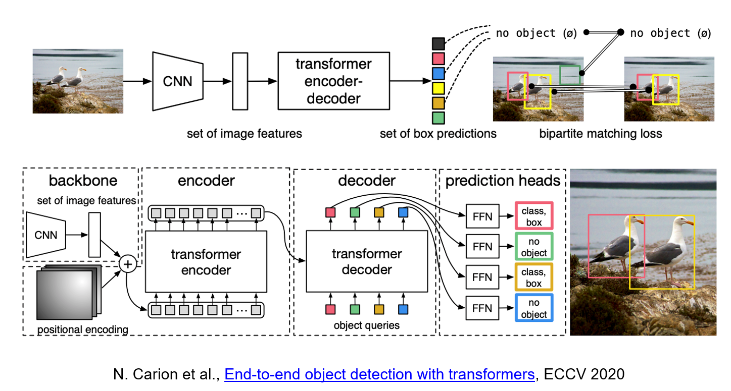
#### Detection Transformer
|
||
|
||
Use transformer architecture to detect the object.
|
||
|
||
|
||
|
||
DETR uses a conventional CNN backbone to learn a 2D representation of an input image. The model flattens it and supplements it with a positional encoding before passing it into a transformer encoder. A transformer decoder then takes as input a small fixed number of learned positional embeddings, which we call object queries, and additionally attends to the encoder output. We pass each output embedding of the decoder to a shared feed forward network (FFN) that predicts either a detection (class and bounding box) or a "no object" class.
|
||
|