NoteNextra-origin/content/CSE5313/CSE5313_L24.md

CSE5313 Coding and information theory for data science (Lecture 24)

Continue on coded computing

!Coded computing scheme

Matrix-vector multiplication: y=Ax, where A\in \mathbb{F}^{M\times N},x\in \mathbb{F}^N

• MDS codes.
  • Recover threshold K=M.
• Short-dot codes.
  • Recover threshold K\geq M.
  • Every node receives at most s=\frac{P-K+M}{P}. N elements of x.

Matrix-matrix multiplication

Problem Formulation:

• A=[A_0 A_1\ldots A_{M-1}]\in \mathbb{F}^{L\times L}, B=[B_0,B_1,\ldots,B_{M-1}]\in \mathbb{F}^{L\times L}
• A_m,B_m are submatrices of A,B.
• We want to compute C=A^\top B.

Trivial solution:

• Index each worker node by m,n\in [0,M-1].
• Worker node (m,n) performs matrix multiplication A_m^\top\cdot B_n.
• Need P=M^2 nodes.
• No erasure tolerance.

Can we do better?

1-D MDS Method

Create [\tilde{A}_0,\tilde{A}_1,\ldots,\tilde{A}_{S-1}] by encoding [A_0,A_1,\ldots,A_{M-1}]. with some (S,M) MDS code.

Need P=SM worker nodes, and index each one by s\in [0,S-1], n\in [0,M-1].

Worker node (s,n) performs matrix multiplication \tilde{A}_s^\top\cdot B_n.

\begin{bmatrix}
A_0^\top\\
A_1^\top\\
A_0^\top+A_1^\top
\end{bmatrix}
\begin{bmatrix}
B_0 & B_1
\enn{bmatrix}

Need S-M responses from each column.

The recovery threshold K=P-S+M nodes.

This is trivially parity check code with 1 recovery threshold.

2-D MDS Method

Encode [A_0,A_1,\ldots,A_{M-1}] with some (S,M) MDS code.

Encode [B_0,B_1,\ldots,B_{M-1}] with some (S,M) MDS code.

Need P=S^2 nodes.

\begin{bmatrix}
A_0^\top\\
A_1^\top\\
A_0^\top+A_1^\top
\end{bmatrix}
\begin{bmatrix}
B_0 & B_1 & B_0+B_1
\enn{bmatrix}

Decodability depends on the pattern.

• Consider an S\times S bipartite graph (rows on left, columns on right).
• Draw an (i,j) edge if \tilde{A}_i^\top\cdot \tilde{B}_j is missing
• Row i is decodable if and only if the degree of $i$'th left node \leq S-M.
• Column j is decodable if and only if the degree of $j$'th right node \leq S-M.

Peeling algorithm:

• Traverse the graph.
• If \exists v,$\deg v\leq S-M$, remove edges.
• Repeat.

Corollary:

• A pattern is decodable if and only if the above graph does not contain a subgraph with all degree larger than S-M.

Note

1. K_{1D-MDS}=P-S+M=\Theta(P) (linearly)
2. K_{2D-MDS}=P-(S-M+1)^2+1.
3. K_{product}<P-M^2=S^2-M^2=\Theta(\sqrt{P})

Our goal is to get rid of P.

Polynomial codes

Polynomial representation

Coefficient representation of a polynomial:

• f(x)=f_dx^d+f_{d-1}x^{d-1}+\cdots+f_1x+f_0
• Uniquely defined by coefficients [f_d,f_{d-1},\ldots,f_0].

Value presentation of a polynomial:

• Theorem: A polynomial of degree d is uniquely determined by d+1 points.
• Proof Outline: First create a polynomial of degree d from the d+1 points using Lagrange interpolation, and show such polynomial is unique.
• Uniquely defined by evaluations [(\alpha_1,f(\alpha_1)),\ldots,(\alpha_{d},f(\alpha_{d}))]

Why should we want value representation?

• With coefficient representation, polynomial product takes O(d^2) multiplications.
• With value representation, polynomial product takes 2d+1 multiplications.

Definition of a polynomial code

link to paper

Problem formulation:

A=[A_0,A_1,\ldots,A_{M-1}]\in \mathbb{F}^{L\times L}, B=[B_0,B_1,\ldots,B_{M-1}]\in \mathbb{F}^{L\times L}

We want to compute C=A^\top B.

Define matrix polynomials:

p_A(x)=\sum_{i=0}^{M-1} A_i x^i, degree M-1

p_B(x)=\sum_{i=0}^{M-1} B_i x^{iM}, degree M(M-1)

where each A_i,B_i are matrices

We have

h(x)=p_A(x)p_B(x)=\sum_{i=0}^{M-1}\sum_{j=0}^{M-1} A_i B_j x^{i+jM}

\deg h(x)\leq M(M-1)+M-1=M^2-1

Observe that

x^{i_1+j_1M}=x^{i_2+j_2M}

if and only if m_1=n_1 and m_2=n_2.

The coefficient of x^{i+jM} is A_i^\top B_j.

Computing C=A^\top B is equivalent to find the coefficient representation of h(x).

Encoding of polynomial codes

The master choose \omega_0,\omega_1,\ldots,\omega_{P-1}\in \mathbb{F}.

• Note that this requires |\mathbb{F}|\geq P.

For every node i\in [0,P-1], the master computes \tilde{A}_i=p_A(\omega_i)

• Equivalent to multiplying [A_0^\top,A_1^\top,\ldots,A_{M-1}^\top] by Vandermonde matrix over \omega_0,\omega_1,\ldots,\omega_{P-1}.
• Can be speed up using FFT.

Similarly, the master computes \tilde{B}_i=p_B(\omega_i) for every node i\in [0,P-1].

Every node i\in [0,P-1] computes and returns c_i=p_A(\omega_i)p_B(\omega_i) to the master.

c_i is the evaluation of polynomial h(x)=p_A(x)p_B(x) at \omega_i.

Recall that h(x)=\sum_{i=0}^{M-1}\sum_{j=0}^{M-1} A_i^\top B_j x^{i+jM}.

• Computing C=A^\top B is equivalent to finding the coefficient representation of h(x).

Recall that a polynomial of degree d can be uniquely defined by d+1 points.

• With MN evaluations of h(x), we can recover the coefficient representation for polynomial h(x).

The recovery threshold K=M^2, independent of P, the number of worker nodes.

Done.

MatDot Codes

link to paper

Problem formulation:

• We want to compute C=A^\top B.

• Unlike polynomial codes, we let $A=\begin{bmatrix} A_0\ A_1\ \vdots\ A_{M-1} \end{bmatrix}$ and $B=\begin{bmatrix} B_0\ B_1\ \vdots\ B_{M-1} \end{bmatrix}$. And A,B\in \mathbb{F}^{L\times L}.

• In polynomial codes, $A=\begin{bmatrix} A_0 A_1\ldots A_{M-1} \end{bmatrix}$ and $B=\begin{bmatrix} B_0 B_1\ldots B_{M-1} \end{bmatrix}$.

Key observation:

A_m^\top is an L\times \frac{L}{M} matrix, and B_m is an \frac{L}{M}\times L matrix. Hence, A_m^\top B_m is an L\times L matrix.

Let C=A^\top B=\sum_{m=0}^{M-1} A_m^\top B_m.

Let p_A(x)=\sum_{m=0}^{M-1} A_m x^m, degree M-1.

Let p_B(x)=\sum_{m=0}^{M-1} B_m x^m, degree M-1.

Both have degree M-1.

And h(x)=p_A(x)p_B(x).

\deg h(x)\leq M-1+M-1=2M-2

Key observation:

• The coefficient of the term x^{M-1} in h(x) is \sum_{m=0}^{M-1} A_m^\top B_m.

Recall that C=A^\top B=\sum_{m=0}^{M-1} A_m^\top B_m.

Finding this coefficient is equivalent to finding the result of A^\top B.

Here we sacrifice the bandwidth of the network for the computational power.

General Scheme for MatDot Codes

The master choose \omega_0,\omega_1,\ldots,\omega_{P-1}\in \mathbb{F}.

• Note that this requires |\mathbb{F}|\geq P.

For every node i\in [0,P-1], the master computes \tilde{A}_i=p_A(\omega_i) and \tilde{B}_i=p_B(\omega_i).

• p_A(x)=\sum_{m=0}^{M-1} A_m x^m, degree M-1.
• p_B(x)=\sum_{m=0}^{M-1} B_m x^m, degree M-1.

The master sends \tilde{A}_i,\tilde{B}_i to node i.

Every node i\in [0,P-1] computes and returns c_i=p_A(\omega_i)p_B(\omega_i) to the master.

The master needs \deg h(x)+1=2M-1 evaluations to obtain h(x).

• The recovery threshold is K=2M-1

Recap on Matrix-Matrix multiplication

A,B\in \mathbb{F}^{L\times L}, we want to compute C=A^\top B with P nodes.

Every node receives \frac{1}{m} of A and \frac{1}{m} of B.

Code	Recovery threshold K
1D-MDS	\Theta(P)
2D-MDS	\leq \Theta(\sqrt{P})
Polynomial codes	\Theta(M^2)
MatDot codes	\Theta(M)

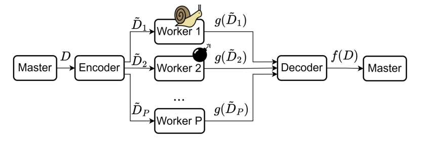
Polynomial Evaluation

Problem formulation:

• We have K datasets X_1,X_2,\ldots,X_K.
• Want to compute some polynomial function f of degree d on each dataset.
  • Want f(X_1),f(X_2),\ldots,f(X_K).
• Examples:
  • X_1,X_2,\ldots,X_K are points in \mathbb{F}^{M\times M}, and f(X)=X^8+3X^2+1.
  • X_k=(X_k^{(1)},X_k^{(2)}), both in \mathbb{F}^{M\times M}, and f(X)=X_k^{(1)}X_k^{(2)}.
  • Gradient computation.

P worker nodes:

• Some are stragglers, i.e., not responsive.
• Some are adversaries, i.e., return erroneous results.
• Privacy: We do not want to expose datasets to worker nodes.

Replication code

Suppose P=(r+1)\cdot K.

• Partition the P nodes to K groups of size r+1 each.
• Node in group i computes and returns f(X_i) to the master.
• Replication tolerates r stragglers, or \lfloor \frac{r}{2} \rfloor adversaries.

Linear codes

However, f is a polynomial of degree d, not a linear transformation unless d=1.

• f(cX)\neq cf(X), where c is a constant.
• f(X_1+X_2)\neq f(X_1)+f(X_2).

Our goal is to create an encoder/decode such that:

• Linear encoding: is the codeword of [X_1,X_2,\ldots,X_K] for some linear code.
• The f(X_i) are decodable from some subset of $f(\tilde{X}_i)$'s.
• $X_i$'s are kept private.

Lagrange Coded Computing

Let \ell(z) be a polynomial whose evaluations at \omega_1,\ldots,\omega_{K} are X_1,\ldots,X_K.

Then every f(X_i)=f(\ell(\omega_i)) is an evaluation of polynomial f\cicc \ell(z) at \omega_i.

If the master obtains the composition h=f\circ \ell, it can obtain every f(X_i)=h(\omega_i).

Goal: The master wished to obtain the polynomial h(z)=f(\ell(z)).

Intuition:

• Encoding is performed by evaluating \ell(z) at \alpha_1,\ldots,\alpha_P\in \mathbb{F}, and P>K for redundancy.
• Nodes apply f on an evaluation of \ell and obtain an evaluation of h.
• The master receives some potentially noisy evaluations, and finds h.
• The master evaluates h at \omega_1,\ldots,\omega_K to obtain f(X_1),\ldots,f(X_K).

Encoding for Lagrange coded computing

Need polynomial \ell(z) such that:

• X_k=\ell(\omega_k) for every k\in [K].

Having obtained such \ell we let \tilde{X}_i=\ell(\alpha_i) for every i\in [P].

\span{\tilde{X}_1,\tilde{X}_2,\ldots,\tilde{X}_P}=\span{\ell_1(x),\ell_2(x),\ldots,\ell_P(x)}.

Want X_k=\ell(\omega_k) for every k\in [K].

Tool: Lagrange interpolation.

• \ell_k(z)=\prod_{i\neq k} \frac{z-\omega_j}{\omega_k-\omega_j}.
• \ell(z)=1 and \ell_k(\omega_k)=0 for every j\neq k.
• \deg \ell(z)=K-1.

Let \ell(z)=\sum_{k=1}^K X_k\ell_k(z).

• \deg \ell=K-1.
• \ell(\omega_k)=X_k for every k\in [K].

Let \tilde{X}_i=\ell(\alpha_i)=\sum_{k=1}^K X_k\ell_k(\alpha_i).

Every \tilde{X}_i is a linear combination of X_1,\ldots,X_K.

(\tilde{X}_1,\tilde{X}_2,\ldots,\tilde{X}_P)=(X_1,\ldots,X_K)\cdot G=(X_1,\ldots,X_K)\begin{bmatrix}
\ell_1(\alpha_1) & \ell_1(\alpha_2) & \cdots & \ell_1(\alpha_P) \\
\ell_2(\alpha_1) & \ell_2(\alpha_2) & \cdots & \ell_2(\alpha_P) \\
\vdots & \vdots & \ddots & \vdots \\
\ell_P(\alpha_1) & \ell_P(\alpha_2) & \cdots & \ell_P(\alpha_P)
\end{bmatrix}

This G is called a Lagrange matrix with respect to

• \omega_1,\ldots,\omega_K. (interpolation points)
• \alpha_1,\ldots,\alpha_P. (evaluation points)

Continue next lecture