8.3 KiB
Math401 Topic 5: Introducing dynamics: classical and non-commutative
Section 1: Dynamics in classical probability
Basic definitions
Definition of orbit
Let T:\Omega\to\Omega be a map (may not be invertible) generating a dynamical system on \Omega. Given \omega\in \Omega, the (forward) orbit of \omega is the set \mathscr{O}(\omega)=\{T^n(\omega)\}_{n\in\mathbb{Z}}.
The theory of dynamics is the study of properties of orbits.
Definition of measure-preserving map
Let P be a probability measure on a $\sigma$-algebra \mathscr{F} of subsets of \Omega. (that is, P:\mathscr{F}\to anything) A measurable transformation T:\Omega\to\Omega is said to be measure-preserving if for all random variables \psi:\Omega\to\mathbb{R}, we have \mathbb{E}(\psi\circ T)=\mathbb{E}(\psi), that is:
\int_\Omega (\psi\circ T)(\omega)dP(\omega)=\int_\Omega \psi(\omega)dP(\omega)
Example:
The doubling map T:\Omega\to\Omega is defined as T(x)=2x\mod 1, is a Lebesgue measure preserving map on \Omega=[0,1].
Definition of isometry
The composition operator \psi\mapsto U\psi=\psi\circ T, where T is a measure preserving map defined on \mathscr{H}=L^2(\Omega,\mathscr{F},P) is isometry of \mathscr{H} if \langle U\psi,U\phi\rangle=\langle\psi,\phi\rangle for all \psi,\phi\in\mathscr{H}.
Definition of unitary
The composition operator \psi\mapsto U\psi=\psi\circ T, where T is a measure preserving map defined on \mathscr{H}=L^2(\Omega,\mathscr{F},P) is unitary of \mathscr{H} if U is an isometry and T is invertible with measurable inverse.
Section 2: Continuous time (classical) dynamical systems
Spring-mass system
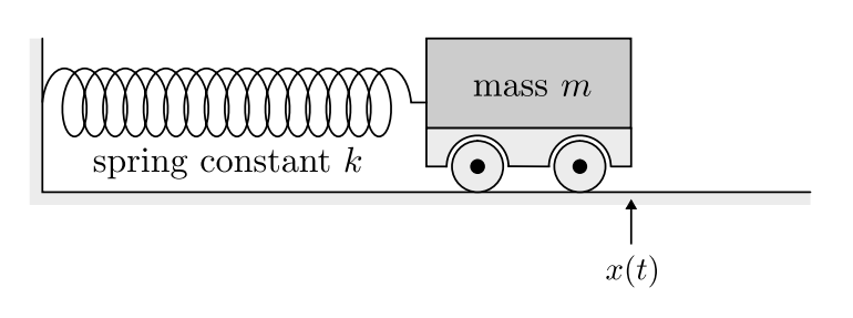
The pure state of the system is given by the position and velocity of the mass. (x,v) is a point in \mathbb{R}^2. \mathbb{R}^2 is the state space of the system. (or phase space)
The motion of the system in its state space is a closed curve.
\Phi_t(x,v)=\left(\cos(\omega t)x-\frac{1}{\omega}\sin(\omega t)v, \cos(\omega t)v-\omega\sin(\omega t)x\right)
Such system with closed curve is called integrable system. Where the doubling map produces orbits having distinct dynamical properties (chaotic system).
Note, some section is intentionally ignored here. They are about in the setting of operators on Hilbert spaces, the evolution of (classical, non-dissipative e.g. linear spring-mass system) system, is implemented by a one-parameter group of unitary operators.
The detailed construction is omitted here.
Definition of Hermitian operator
A linear operator A on a Hilbert space \mathscr{H} is said to be Hermitian if \forall \psi,\phi\in domain of $A$, we have \langle A\psi,\phi\rangle=\langle\psi,A\phi\rangle.
It is skew-Hermitian if \langle A\psi,\phi\rangle=-\langle\psi,A\phi\rangle.
Section 3: Hamiltonians and the Schrödinger equation (finite dimensional version)
the problem of solving Schrödinger equation is at its core about studying the spectral theory of the Hamiltonian operator.
Dynamics in 2-dimensional (2 level) systems (qubit)
In previous sections, we know that any self-adjoint matrix has the form x_0+\vec{x}\cdot \sigma, where \sigma is the Pauli matrices.
And (x_0,\vec{x})\in\mathbb{R}^4 is a point in \mathbb{R}^4.
The general form (time-independent) of the Hamiltonian for a 2-level system is:
H=\begin{pmatrix}
x_0+x_3 & x_1-ix_2 \\
x_1+ix_2 & -x_0+x_3
\end{pmatrix}
Parameterizing the curves in Bloch space generated by Hamiltonian. In physical dimension of \vec{x}=\omega\hbar\vec{s}, \omega>0. \omega\hbar is the physical dimension of energy.
we have:
H=\omega\hbar\begin{pmatrix}
s_3 & s_1-is_2 \\
s_1+is_2 & -s_3
\end{pmatrix}
[Continue on the orbits of states in the Bloch sphere] skip for now.
Section 4: Transition probability, probability amplitudes and the Born rule
the modulus squared of a probability amplitude is the probability of the corresponding state.
Basic definitions in transition probability
Definition of probability amplitude
For a n-dimensional Hilbert space \mathscr{H}, the system is initially in a pure state give by the unit vector |\psi_0\rangle\in\mathscr{H}, thus with the density operator \rho_0=|\psi_0\rangle\langle\psi_0|.
Then the state at time t_1 is given by |\psi_1\rangle=A|\psi_0\rangle, where A\in U(n) is a unitary operator.
Then the density operator at time t_1 is given by \rho_1=|\psi_1\rangle\langle\psi_1|=A|\psi_0\rangle\langle\psi_0|A^*=A\rho_0A^*.
The entry of A are a_{ij}=\langle i|A|j\rangle. where |i\rangle is the basis of \mathscr{H}.
The a_{ij} are the probability amplitudes of the transition from state |i\rangle to state |j\rangle.
Definition of transition probability
Given above, the transition probability from state |i\rangle to state |j\rangle is given by:
|a_{ij}|^2
Sum over paths
To each path of classical states, path j\to i: i_0=j,i_1,i_2,\cdots,i_l=i, we associates the probability amplitude of the path given by:
|\text{path}(j\to i)\rangle=\langle i_0|i_1\rangle\langle i_1|i_2\rangle\cdots\langle i_{l-1}|i_l\rangle
The probability of the path is given by:
\operatorname{Prob}(i|j)=\left|\sum_{\text{all paths}j\to i \text{ with } l \text{ steps}}|\text{path}(j\to i)\rangle\right|^2
Measuring a qubit
Definition of qubit
A qubit is a 2-level quantum system.
One example of qubit is the photon polarization.
Measurement of a qubit
The measurement of a qubit is a map fro the space of density operators, to a point on the intervals [0,1].
This gives a probability distribution on the interval [0,1] in our classical probability space.
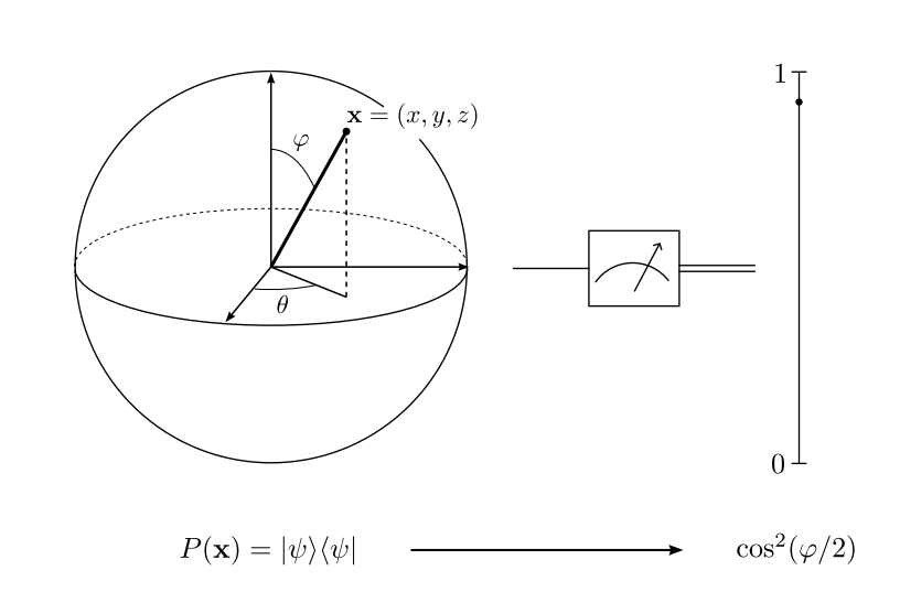
Here p=\cos^2(\theta)\in[0,1]. is the probability of the state being in the state |0\rangle.
The north pole on the Bloch sphere gives probability 1 for the state being in the state |0\rangle.
The south pole on the Bloch sphere gives probability 1 for the state being in the state |1\rangle.
The equator on the Bloch sphere gives probability 1/2 for the state being in the state |0\rangle or |1\rangle.
Projective measurement of an $N$-qubit system
For N qubits, the pure quantum state \rho=|\psi\rangle\langle\psi| represented by the state vector |\psi\rangle\in\mathscr{H}^{\otimes N}=\mathscr{H}\otimes\cdots\otimes\mathscr{H}(\mathscr{H}=\mathbb{C}^2).
This produces as output the random variable X\in \{0,1\}^N. X=(a_1,a_2,\cdots,a_N), where a_i\in \{0,1\}.
By the Born rule,
\operatorname{Prob}(X=(a_1,a_2,\cdots,a_N))=\left|\langle a_1a_2\cdots a_N|\psi\rangle\right|^2
where \langle a_1a_2\cdots a_N|\psi\rangle=\langle a_1|\otimes\langle a_2|\otimes\cdots\otimes\langle a_N|\psi\rangle.
The input vector state |\psi\rangle is a unit vector in \mathscr{H}^{\otimes N}.
This can be written as a tensor product of the basis vectors:
|\psi\rangle=\sum_{a_1,a_2,\cdots,a_N} c_{a_1,a_2,\cdots,a_N}|a_1a_2\cdots a_N\rangle
where c_{a_1,a_2,\cdots,a_N}\in\mathbb{C}.
The probability distribution of the post-measurement classical random variable X can be represented as a point in the 2^N-1 dimensional simplex of all probability distributions on the set \{0,1\}^N.
\mathscr{P}(\{0,1\}^N)=\left\{(p_1,p_2,\cdots,p_{2^N})\in\mathbb{R}^{2^N}:p_i\geq 0,\sum_{i=1}^{2^N}p_i=1\right\}

here we use the binary representation for the index i in the diagram.
Pure versus mixed states
A pure state is a state that is represented by a unit vector in \mathscr{H}^{\otimes N}.
A mixed state is a state that is represented by a density operator in \mathscr{H}^{\otimes N}. (convex combination of pure states)
if \rho_j=|\psi_j\rangle\langle\psi_j|, then \rho=\sum_{j=1}^N p_j\rho_j is a mixed state, where p_j\geq 0 and \sum_{j=1}^N p_j=1.
Projective measurement of subsystem and partial trace
This section is related to quantum random walk and we will skip it for now.
Section 5: Quantum random walk
This part is skipped, it is an interesting topic, but it is not the focus of my research for now.