Compare commits
5 Commits
distribute
...
dev-test
| Author | SHA1 | Date | |
|---|---|---|---|
|
|
760f7cb26d | ||
|
|
c9c119e991 | ||
|
|
e4995c8118 | ||
|
|
f89b3cb70d | ||
|
|
f8df23526b |
73
.github/workflows/sync-from-gitea-deploy.yml
vendored
73
.github/workflows/sync-from-gitea-deploy.yml
vendored
@@ -1,73 +0,0 @@
|
||||
name: Sync from Gitea (distribute→distribute, keep workflow)
|
||||
|
||||
on:
|
||||
schedule:
|
||||
# 2 times per day (UTC): 7:00, 11:00
|
||||
- cron: '0 7,11 * * *'
|
||||
workflow_dispatch: {}
|
||||
|
||||
permissions:
|
||||
contents: write # allow pushing with GITHUB_TOKEN
|
||||
|
||||
jobs:
|
||||
mirror:
|
||||
runs-on: ubuntu-latest
|
||||
|
||||
steps:
|
||||
- name: Check out GitHub repo
|
||||
uses: actions/checkout@v4
|
||||
with:
|
||||
fetch-depth: 0
|
||||
|
||||
- name: Fetch from Gitea
|
||||
env:
|
||||
GITEA_URL: ${{ secrets.GITEA_URL }}
|
||||
GITEA_USER: ${{ secrets.GITEA_USERNAME }}
|
||||
GITEA_TOKEN: ${{ secrets.GITEA_TOKEN }}
|
||||
run: |
|
||||
# Build authenticated Gitea URL: https://USER:TOKEN@...
|
||||
AUTH_URL="${GITEA_URL/https:\/\//https:\/\/$GITEA_USER:$GITEA_TOKEN@}"
|
||||
|
||||
git remote add gitea "$AUTH_URL"
|
||||
git fetch gitea --prune
|
||||
|
||||
- name: Update distribute from gitea/distribute, keep workflow, and force-push
|
||||
env:
|
||||
GH_TOKEN: ${{ secrets.GITHUB_TOKEN }}
|
||||
GH_REPO: ${{ github.repository }}
|
||||
run: |
|
||||
# Configure identity for commits made by this workflow
|
||||
git config user.name "github-actions[bot]"
|
||||
git config user.email "github-actions[bot]@users.noreply.github.com"
|
||||
|
||||
# Authenticated push URL for GitHub
|
||||
git remote set-url origin "https://x-access-token:${GH_TOKEN}@github.com/${GH_REPO}.git"
|
||||
|
||||
WF_PATH=".github/workflows/sync-from-gitea.yml"
|
||||
|
||||
# If the workflow exists in the current checkout, save a copy
|
||||
if [ -f "$WF_PATH" ]; then
|
||||
mkdir -p /tmp/gh-workflows
|
||||
cp "$WF_PATH" /tmp/gh-workflows/
|
||||
fi
|
||||
|
||||
# Reset local 'distribute' to exactly match gitea/distribute
|
||||
if git show-ref --verify --quiet refs/remotes/gitea/distribute; then
|
||||
git checkout -B distribute gitea/distribute
|
||||
else
|
||||
echo "No gitea/distribute found, nothing to sync."
|
||||
exit 0
|
||||
fi
|
||||
|
||||
# Restore the workflow into the new HEAD and commit if needed
|
||||
if [ -f "/tmp/gh-workflows/sync-from-gitea.yml" ]; then
|
||||
mkdir -p .github/workflows
|
||||
cp /tmp/gh-workflows/sync-from-gitea.yml "$WF_PATH"
|
||||
git add "$WF_PATH"
|
||||
if ! git diff --cached --quiet; then
|
||||
git commit -m "Inject GitHub sync workflow"
|
||||
fi
|
||||
fi
|
||||
|
||||
# Force-push distribute so GitHub mirrors Gitea + workflow
|
||||
git push origin distribute --force
|
||||
73
.github/workflows/sync-from-gitea.yml
vendored
73
.github/workflows/sync-from-gitea.yml
vendored
@@ -1,73 +0,0 @@
|
||||
name: Sync from Gitea (main→main, keep workflow)
|
||||
|
||||
on:
|
||||
schedule:
|
||||
# 2 times per day (UTC): 7:00, 11:00
|
||||
- cron: '0 7,11 * * *'
|
||||
workflow_dispatch: {}
|
||||
|
||||
permissions:
|
||||
contents: write # allow pushing with GITHUB_TOKEN
|
||||
|
||||
jobs:
|
||||
mirror:
|
||||
runs-on: ubuntu-latest
|
||||
|
||||
steps:
|
||||
- name: Check out GitHub repo
|
||||
uses: actions/checkout@v4
|
||||
with:
|
||||
fetch-depth: 0
|
||||
|
||||
- name: Fetch from Gitea
|
||||
env:
|
||||
GITEA_URL: ${{ secrets.GITEA_URL }}
|
||||
GITEA_USER: ${{ secrets.GITEA_USERNAME }}
|
||||
GITEA_TOKEN: ${{ secrets.GITEA_TOKEN }}
|
||||
run: |
|
||||
# Build authenticated Gitea URL: https://USER:TOKEN@...
|
||||
AUTH_URL="${GITEA_URL/https:\/\//https:\/\/$GITEA_USER:$GITEA_TOKEN@}"
|
||||
|
||||
git remote add gitea "$AUTH_URL"
|
||||
git fetch gitea --prune
|
||||
|
||||
- name: Update main from gitea/main, keep workflow, and force-push
|
||||
env:
|
||||
GH_TOKEN: ${{ secrets.GITHUB_TOKEN }}
|
||||
GH_REPO: ${{ github.repository }}
|
||||
run: |
|
||||
# Configure identity for commits made by this workflow
|
||||
git config user.name "github-actions[bot]"
|
||||
git config user.email "github-actions[bot]@users.noreply.github.com"
|
||||
|
||||
# Authenticated push URL for GitHub
|
||||
git remote set-url origin "https://x-access-token:${GH_TOKEN}@github.com/${GH_REPO}.git"
|
||||
|
||||
WF_PATH=".github/workflows/sync-from-gitea.yml"
|
||||
|
||||
# If the workflow exists in the current checkout, save a copy
|
||||
if [ -f "$WF_PATH" ]; then
|
||||
mkdir -p /tmp/gh-workflows
|
||||
cp "$WF_PATH" /tmp/gh-workflows/
|
||||
fi
|
||||
|
||||
# Reset local 'main' to exactly match gitea/main
|
||||
if git show-ref --verify --quiet refs/remotes/gitea/main; then
|
||||
git checkout -B main gitea/main
|
||||
else
|
||||
echo "No gitea/main found, nothing to sync."
|
||||
exit 0
|
||||
fi
|
||||
|
||||
# Restore the workflow into the new HEAD and commit if needed
|
||||
if [ -f "/tmp/gh-workflows/sync-from-gitea.yml" ]; then
|
||||
mkdir -p .github/workflows
|
||||
cp /tmp/gh-workflows/sync-from-gitea.yml "$WF_PATH"
|
||||
git add "$WF_PATH"
|
||||
if ! git diff --cached --quiet; then
|
||||
git commit -m "Inject GitHub sync workflow"
|
||||
fi
|
||||
fi
|
||||
|
||||
# Force-push main so GitHub mirrors Gitea + workflow
|
||||
git push origin main --force
|
||||
1
.gitignore
vendored
1
.gitignore
vendored
@@ -143,7 +143,6 @@ analyze/
|
||||
|
||||
# pagefind postbuild
|
||||
public/_pagefind/
|
||||
public/sitemap.xml
|
||||
|
||||
# npm package lock file for different platforms
|
||||
package-lock.json
|
||||
@@ -1,7 +1,7 @@
|
||||
# Source: https://github.com/vercel/next.js/blob/canary/examples/with-docker-multi-env/docker/production/Dockerfile
|
||||
# syntax=docker.io/docker/dockerfile:1
|
||||
|
||||
FROM node:20-alpine AS base
|
||||
FROM node:18-alpine AS base
|
||||
|
||||
ENV NODE_OPTIONS="--max-old-space-size=8192"
|
||||
|
||||
|
||||
@@ -28,11 +28,3 @@ Considering the memory usage for this project, it is better to deploy it as sepa
|
||||
```bash
|
||||
docker-compose up -d -f docker/docker-compose.yaml
|
||||
```
|
||||
|
||||
### Snippets
|
||||
|
||||
Update dependencies
|
||||
|
||||
```bash
|
||||
npx npm-check-updates -u
|
||||
```
|
||||
@@ -83,7 +83,7 @@ export default async function RootLayout({ children }) {
|
||||
docsRepositoryBase="https://github.com/Trance-0/NoteNextra/tree/main"
|
||||
sidebar={{ defaultMenuCollapseLevel: 1 }}
|
||||
pageMap={pageMap}
|
||||
// TODO: fix local search with distributed search index over containers
|
||||
// TODO: fix algolia search
|
||||
search={<AlgoliaSearch/>}
|
||||
>
|
||||
{children}
|
||||
|
||||
@@ -9,7 +9,7 @@ import '@docsearch/css';
|
||||
function AlgoliaSearch () {
|
||||
const {theme, systemTheme} = useTheme();
|
||||
const darkMode = theme === 'dark' || (theme === 'system' && systemTheme === 'dark');
|
||||
// console.log("darkMode", darkMode);
|
||||
console.log("darkMode", darkMode);
|
||||
return (
|
||||
<DocSearch
|
||||
appId={process.env.NEXT_SEARCH_ALGOLIA_APP_ID || 'NKGLZZZUBC'}
|
||||
|
||||
@@ -108,7 +108,7 @@ export const ClientNavbar: FC<{
|
||||
item => !('href' in item)
|
||||
).map(item => item.title)
|
||||
)
|
||||
// console.log(existingCourseNames)
|
||||
console.log(existingCourseNames)
|
||||
|
||||
// filter out elements in topLevelNavbarItems with url but have title in existingCourseNames
|
||||
const filteredTopLevelNavbarItems = topLevelNavbarItems.filter(item => !('href' in item && existingCourseNames.has(item.title)))
|
||||
@@ -117,7 +117,7 @@ export const ClientNavbar: FC<{
|
||||
// use filteredTopLevelNavbarItems to generate items
|
||||
const items = filteredTopLevelNavbarItems
|
||||
|
||||
// console.log(filteredTopLevelNavbarItems)
|
||||
console.log(filteredTopLevelNavbarItems)
|
||||
const themeConfig = useThemeConfig()
|
||||
|
||||
const pathname = useFSRoute()
|
||||
@@ -184,4 +184,4 @@ export const ClientNavbar: FC<{
|
||||
</Button>
|
||||
</>
|
||||
)
|
||||
}
|
||||
}
|
||||
|
||||
@@ -1,148 +0,0 @@
|
||||
# CSE332S Object-Oriented Programming in C++ (Lecture 1)
|
||||
|
||||
## Today:
|
||||
|
||||
1. A bit about me
|
||||
2. A bit about the course
|
||||
3. A bit about C++
|
||||
4. How we will learn
|
||||
5. Canvas tour and course policies
|
||||
6. Piazza tour
|
||||
7. Studio: Setup our work environment
|
||||
|
||||
## A bit about me:
|
||||
|
||||
This is my 14th year at WashU.
|
||||
|
||||
- 5 as a graduate student advised by Dr. Cytron
|
||||
- Research focused on optimizing the memory system for garbage collected languages
|
||||
- My 9th as an instructor
|
||||
- Courses taught: 131, 247, 332S, 361S, 422S, 433S, 454A, 523S
|
||||
|
||||
## CSE 332S Overview:
|
||||
|
||||
This course has 3 high level goals:
|
||||
|
||||
1. Gain proficiency with a 2nd programming language
|
||||
2. Introduce important lower-level constructs that many high-level languages abstract away (pointers, explicit dynamic memory management, code compilation, stack management, static programming languages, etc.)
|
||||
3. Teach fundamental object-oriented programming principles and design
|
||||
|
||||
C++ allows us to accomplish all three goals above!
|
||||
|
||||
### An introduction to C++
|
||||
|
||||
C++ is a multi-paradigm language
|
||||
|
||||
- Procedural programming - functions
|
||||
- Object-oriented programming - classes and structs
|
||||
- Generic programming - templates
|
||||
|
||||
C++ is built upon C, keeping lower-level features of C while adding higher-level features
|
||||
|
||||
#### Evolution of C++
|
||||
|
||||
1. C is a procedural programming language primarily used to develop low-level systems software, such as operating systems.
|
||||
- designed to map efficiently to typical machine instructions, making compilation fairly straightforward and giving low-level access to memory
|
||||
- However, type safe code reuse is hard without high-level programming constructs such as objects and generics.
|
||||
2. Stroustrup first designed C++ with classes/objects, but kept procedural parts similar to C
|
||||
3. Templates (generics) were later added and the STL was developed
|
||||
4. C++ is now standardized, with the latest revision of the standard being C++23
|
||||
|
||||
### So, why C++? And an overview of the semester timeline...
|
||||
|
||||
1. C++ allows us to explore programming constructs such as low-level memory access (pointers and references), function calls (stack management), and explicit memory management (1st 1/3rd of the semester)
|
||||
2. We can then learn how those lower-level constructs are used to enable more abstract higher-level constructs, such as objects and the development of the C++ Standard Template Library (the STL) (middle 1/3rd of the semester)
|
||||
3. Finally, we will use C++ to study the fundamentals of object-oriented design (final 3rd of the semester)
|
||||
|
||||
### How we will learn (flipped classroom):
|
||||
|
||||
#### Prior to class
|
||||
|
||||
Lectures are pre-recorded and posted for you to view asynchronously before class
|
||||
|
||||
- Posted 72 hours before class on Canvas
|
||||
|
||||
Post-lecture tasks are posted alongside the lectures and should be completed before class
|
||||
|
||||
- Canvas discussion to ask questions, “like” already asked questions
|
||||
- A short quiz over the lecture content
|
||||
|
||||
#### During class
|
||||
|
||||
- Work on a studio within a group to build an understanding of the topic via hands-on exercises and discussion (10:30 - 11:20 AM, 1:30 - 2:20 PM)
|
||||
- Treat studio as a time to explore and test your understanding of a concept. Place emphasis on exploration.
|
||||
- TAs and I will be there to help guide you through and discuss the exercises.
|
||||
- Optional recitation for the first 30 minutes of each class - content generally based on questions posed in the discussion board. Recitations will be recorded.
|
||||
|
||||
#### Outside of class
|
||||
|
||||
- Readings provide further details on the topics covered in class
|
||||
- Lab assignments ask you to apply the concepts you have learned
|
||||
|
||||
### In-class studio policy
|
||||
|
||||
You should be in-class by 35 minutes after the official class start time (10 am -> 10:35 AM, 1 PM -> 1:35 PM) to receive credit
|
||||
|
||||
- Credit awarded for being in-class and working on studio. If you do not finish the studio, you will still get credit IF you are working on studio
|
||||
- All studio content is fair game on an exam. The exam is hard, the best way to prep is to spend class time efficiently working through studio
|
||||
- If instructors (myself or TAs) feel you are not working on studio, credit will be taken away. Old studios may be reviewed if this is a consistent problem
|
||||
- You should always commit and push the work you completed at the end of class. You should always accept the assignment link and join the team you are working with so you have access to the studio repository.
|
||||
|
||||
### Other options for studio
|
||||
|
||||
If studio must be missed for some reason:
|
||||
|
||||
- Complete the studio exercises in full (must complete all non-optional exercises) within 4 days of the assigned date to receive credit
|
||||
- Friday at 11:59 PM for Monday studios
|
||||
- Sunday at 11:59 PM for Wednesday studios
|
||||
- Ok to work asynchronously in a group
|
||||
|
||||
### Topics we will cover:
|
||||
|
||||
- C++ program basics
|
||||
- Variables, types, control statements, development environments
|
||||
- C++ functions
|
||||
- Parameters, the call stack, exception handling
|
||||
- C++ memory
|
||||
- Addressing, layout, management
|
||||
- C++ classes and structs
|
||||
- Encapsulation, abstraction, inheritance
|
||||
- C++ STL
|
||||
- Containers, iterators, algorithms, functors
|
||||
- OO design
|
||||
- Principles and Fundamentals, reusable design patterns
|
||||
|
||||
### Other details:
|
||||
|
||||
We will use Canvas to distribute lecture slides, studios, assignments, and announcements. Piazza will be used for discussion
|
||||
|
||||
### Lab details:
|
||||
|
||||
CSE 332 focuses on correctness, but also code readability and maintainability
|
||||
|
||||
- Labs graded on correctness as well as programming style
|
||||
- Each lab lists the programming guidelines that should be followed
|
||||
- Please review the CSE 332 programming guidelines before turning in each lab
|
||||
|
||||
Labs 1, 2, and 3 are individual assignments. You may work in groups of up to three on labs 4 and 5
|
||||
|
||||
### Academic Integrity
|
||||
|
||||
Cheating is the misrepresentation of someone else’s work as your own, or assisting someone else in cheating
|
||||
|
||||
- Providing or receiving answers on exams
|
||||
- Accessing unapproved sources of information on an exam
|
||||
- Submitting code written outside of this course in this semester, written by someone else not on your team (or taken from the internet)
|
||||
- Allowing another student to copy your solution
|
||||
- Do not host your projects in public repos
|
||||
|
||||
Please also refer to the McKelvey Academic Integrity Policy
|
||||
|
||||
Online resources may be used to lookup general purpose C++ information (libraries, etc.). They should not be used to lookup questions specific to a course assignment. Any online resources used, including generative AIs such as chatGPT must be cited, with a description of the prompt/question asked. A comment in your code works fine for this. You may use code from the textbook or from [cppreference.com](https://en.cppreference.com/w/) or [cplusplus.com](https://cplusplus.com/) without citations.
|
||||
|
||||
If you have any doubt at all, ask me!
|
||||
|
||||
### Studio: Setting up our working environment
|
||||
|
||||
Visit the course canvas page, sign up for the course piazza page, and get started on studio 1
|
||||
|
||||
@@ -1,274 +0,0 @@
|
||||
# CSE332S Object-Oriented Programming in C++ (Lecture 10)
|
||||
|
||||
## Associative Containers
|
||||
|
||||
| Container | Sorted | Unique Key | Allow duplicates |
|
||||
| -------------------- | ------ | ---------- | ---------------- |
|
||||
| `set` | Yes | Yes | No |
|
||||
| `multiset` | Yes | Yes | Yes |
|
||||
| `unordered_set` | No | Yes | No |
|
||||
| `unordered_multiset` | No | Yes | Yes |
|
||||
| `map` | Yes | Yes | No |
|
||||
| `multimap` | Yes | Yes | Yes |
|
||||
| `unordered_map` | No | Yes | No |
|
||||
| `unordered_multimap` | No | Yes | Yes |
|
||||
|
||||
Associative containers support efficient key lookup
|
||||
vs. sequence containers, which lookup by position
|
||||
Associative containers differ in 3 design dimensions
|
||||
|
||||
- Ordered vs. unordered (tree vs. hash structured)
|
||||
- We’ll look at ordered containers today, unordered next time
|
||||
- Set vs. map (just the key or the key and a mapped type)
|
||||
- Unique vs. multiple instances of a key
|
||||
|
||||
### Ordered Associative Containers
|
||||
|
||||
Example: `set`, `multiset`, `map`, `multimap`
|
||||
|
||||
Ordered associative containers are tree structured
|
||||
- Insert/delete maintain sorted order, e.g. `operator<`
|
||||
- Don’t use sequence algorithms like `sort` or `find` with them
|
||||
- Already sorted, so sorting unnecessary (or harmful)
|
||||
- `find` is more efficient (logarithmic time) as a container method
|
||||
Ordered associative containers are bidirectional
|
||||
- Can iterate through them in either direction, find sub-ranges
|
||||
- Can use as source or destination for algorithms like `copy`
|
||||
|
||||
### Set vs. Map
|
||||
|
||||
A set/multiset stores keys (the key is the entire value)
|
||||
|
||||
- Used to collect single-level information (e.g., a set of words to ignore)
|
||||
- Avoid in-place modification of keys (especially in a set or multiset)
|
||||
|
||||
A map/multimap associates keys with mapped types
|
||||
|
||||
- That style of data structure is sometimes called an associative array
|
||||
- Map subscripting operator takes key, returns reference to mapped type
|
||||
- E.g., `string s = employees[id]; // returns employee name`
|
||||
- If key does not exist, `[]` creates new entry with the key, value-initialized (0 if numeric, default initialized if class) instance of the mapped type
|
||||
|
||||
### Unique vs. Multiple Instances of a Key
|
||||
|
||||
In set and map containers, keys are unique
|
||||
|
||||
- In set, keys are the entire value, so every element is unique
|
||||
- In map, multiple keys may map to same value, but can’t duplicate keys
|
||||
- Attempt to insert a duplicate key is ignored by the container (returns false)
|
||||
|
||||
In multiset and multimap containers, duplicate keys ok
|
||||
|
||||
- Since containers are ordered, duplicates are kept next to each other
|
||||
- Insertion will always succeed, at appropriate place in the order
|
||||
|
||||
### Key Types, Comparators, Strict Weak Ordering
|
||||
|
||||
Like `sort` algorithm, can modify container’s order ...
|
||||
... with any callable object that can be used correctly for sort
|
||||
|
||||
Must establish a **strict weak ordering** over elements
|
||||
|
||||
- Two keys cannot both be less than each other (inequality), so comparison operator must return `false` if they are equal
|
||||
- If `a < b` and `b < c` then `a < c` (transitivity of inequality)
|
||||
- If `!(a < b)` and `! (b < a)` then `a == b` (equivalence)
|
||||
- If `a == b` and `b == c` then `a == c` (transitivity of eqivalence)
|
||||
|
||||
_Sounds like definition of order in math_
|
||||
|
||||
Type of the callable object is used in container type
|
||||
|
||||
- Cool example in LLM pp. 426 using `decltype` for a function
|
||||
- Could do this by declaring your own pointer to function type
|
||||
- But much easier to let compiler’s type inference figure it out for you
|
||||
|
||||
### Pairs
|
||||
|
||||
Maps use `pair` template to hold key, mapped type
|
||||
|
||||
- A `pair` can be used hold any two types
|
||||
- Maps use the key type as the 1st element of the pair (`p.first`)
|
||||
- Maps use the mapped type as the 2nd element of the pair (`p.second`)
|
||||
|
||||
Can compare `pair` variables using operators
|
||||
|
||||
- Equivalence, less than, other relational operators
|
||||
|
||||
Can declare `pair` variables several different ways
|
||||
|
||||
- Easiest uses initialization list (curly braces around values) (e.g. `pair<string, int> p = {"hello", 1};`)
|
||||
- Can also default construct (value initialization) (e.g. `pair<string, int> p;`)
|
||||
- Can also construct with two values (e.g. `pair<string, int> p("hello", 1);`)
|
||||
- Can also use special `make_pair` function (e.g. `pair<string, int> p = make_pair("hello", 1);`)
|
||||
|
||||
### Unordered Containers (UCs)
|
||||
|
||||
Example: `unordered_set`, `unordered_multiset`, `unordered_map`, `unordered_multimap`
|
||||
|
||||
UCs use `==` to compare elements instead of `<` to order them
|
||||
|
||||
- Types in unordered containers must be equality comparable
|
||||
- When you write your own structs, overload `==` as well as `<`
|
||||
|
||||
UCs store elements in indexed buckets instead of in a tree
|
||||
|
||||
- Useful for types that don’t have an obvious ordering relation over their values
|
||||
|
||||
UCs use hash functions to put and find elements in buckets
|
||||
|
||||
- May improve performance in some cases (if performance profiling suggests so)
|
||||
- Declare UCs with pluggable hash functions via callable objects, decltype, etc.
|
||||
- Or specialize the `std::hash()` template for your type, used by default
|
||||
|
||||
### Summary
|
||||
|
||||
Use associative containers for key based lookup
|
||||
|
||||
- Ordering of elements is maintained over the keys
|
||||
- Think ranges and ordering rather than position indexes
|
||||
- A sorted vector may be a better alternative (depends on which operations you will use most often, and their costs)
|
||||
|
||||
Ordered associative containers use strict weak order
|
||||
|
||||
- Operator `<` or any callable object that acts like `<` over `int` can be used
|
||||
|
||||
Maps allow two-level (dictionary-like) lookup
|
||||
|
||||
- Vs. sets which are used for “there or not there” lookup
|
||||
- Map uses a `pair` to associate key with mapped type
|
||||
|
||||
Can enforce uniqueness or allow duplicates
|
||||
|
||||
- Duplicates are still stored in order, creating “equal ranges”
|
||||
|
||||
## IO Libraries
|
||||
|
||||
### `std::copy()`
|
||||
|
||||
`std::copy()`
|
||||
|
||||
http://www.cplusplus.com/reference/algorithm/copy/
|
||||
|
||||
Takes 3 parameters:
|
||||
|
||||
- `copy(InputIterator first, InputIterator last, OutputIterator result);`
|
||||
- `[first, last)` specifies the range of elements to copy.
|
||||
- `result` specifies where we are copying to.
|
||||
|
||||
Example:
|
||||
|
||||
```cpp
|
||||
vector<int> v = {1, 2, 3, 4, 5};
|
||||
// copy v to cout
|
||||
std::copy(v.begin(), v.end(), std::ostream_iterator<int>(std::cout, " "));
|
||||
```
|
||||
|
||||
Some useful destination iterator types:
|
||||
|
||||
1. `ostream_iterator` - iterator over an output stream (like `cout`)
|
||||
2. `insert_iterator` - inserts elements directly into an STL container (will be practiced in studio)
|
||||
|
||||
```cpp
|
||||
#include <iostream>
|
||||
#include <string>
|
||||
#include <fstream>
|
||||
#include <iterator>
|
||||
#include <algorithm>
|
||||
|
||||
using namespace std;
|
||||
|
||||
int main(int argc, char *argv[]) {
|
||||
if (argc != 3) {
|
||||
cerr << "Usage: " << argv[0] << " <input file> <output file>" << endl;
|
||||
return 1;
|
||||
}
|
||||
|
||||
string input_file = argv[1];
|
||||
string output_file = argv[2];
|
||||
|
||||
ifstream input_file(input_file.c_str());
|
||||
ofstream output_file(output_file.c_str());
|
||||
|
||||
// don't skip whitespace
|
||||
input_file >> noskipws;
|
||||
|
||||
istream_iterator<char> i (input_file);
|
||||
ostream_iterator<char> o (output_file);
|
||||
|
||||
// copy the input file to the output file: copy(InputIterator first, InputIterator last, OutputIterator result);
|
||||
copy(i, istream_iterator<char>(), o);
|
||||
|
||||
cout << "Copied input file" << input_file << " to " << output_file << endl;
|
||||
|
||||
return 0;
|
||||
}
|
||||
```
|
||||
|
||||
### IO reviews
|
||||
|
||||
How to move data into and out of a program:
|
||||
|
||||
- Using `argc` and `argv` to pass command line args
|
||||
- Using `cout` to print data out to the terminal
|
||||
- Using `cin` to obtain data from the user at run-time
|
||||
- Using an `ifstream` to read data in from a file
|
||||
- Using an `ofstream` to write data out to a file
|
||||
|
||||
How to move data between strings, basic types
|
||||
|
||||
- Using an `istringstream` to extract formatted int values
|
||||
- Using an `ostringstream` to assemble a string
|
||||
|
||||
### Streams
|
||||
|
||||
Simply a buffer of data (array of bytes).
|
||||
|
||||
Insertion operator (`<<`) specifies how to move data from a variable into an output stream
|
||||
Extraction operator (`>>`) specifies how to pull data off of an input stream and store it into a variable
|
||||
|
||||
Both operators defined for built-in types:
|
||||
|
||||
- Numeric types
|
||||
- Pointers
|
||||
- Pointers to char (char *)
|
||||
|
||||
Cannot copy or assign stream objects
|
||||
|
||||
- Copy construction or assignment syntax using them results in a compile-time error
|
||||
|
||||
Extraction operator consumes data from input stream
|
||||
|
||||
- "Destructive read" that reads a different element each time
|
||||
- Use a variable if you want to read same value repeatedly
|
||||
|
||||
Need to test streams’ condition states
|
||||
|
||||
- E.g., calling the `is_open` method on a file stream
|
||||
- E.g., use the stream object in a while or if test
|
||||
- Insertion and extraction operators return a reference to a stream object, so can test them too
|
||||
|
||||
File stream destructor calls close automatically
|
||||
|
||||
### Flushing and stream manipulators
|
||||
|
||||
An output stream may hold onto data for a while, internally
|
||||
|
||||
- E.g., writing chunks of text rather than a character at a time is efficient
|
||||
- When it writes data out (e.g., to a file, the terminal window, etc.) is entirely up to the stream, **unless you tell it to flush out its buffers**
|
||||
- If a program crashes, any un-flushed stream data is lost
|
||||
- So, flushing streams reasonably often is an excellent debugging trick
|
||||
|
||||
Can tie an input stream directly to an output stream
|
||||
|
||||
- Output stream is then flushed by call to input stream extraction operator
|
||||
- E.g., `my_istream.tie(&my_ostream);`
|
||||
- `cout` is already tied to `cin` (useful for prompting the user, getting input)
|
||||
|
||||
Also can flush streams directly using stream manipulators
|
||||
|
||||
- E.g., `cout << flush;` or `cout << endl;` or `cout << unitbuf;`
|
||||
|
||||
Other stream manipulators are useful for formatting streams
|
||||
|
||||
- Field layout: `setwidth`, `setprecision`, etc.
|
||||
- Display notation: `oct`, `hex`, `dec`, `boolalpha`, `nobooleanalpha`, `scientific`, etc.
|
||||
@@ -1,171 +0,0 @@
|
||||
# CSE332S Object-Oriented Programming in C++ (Lecture 11)
|
||||
|
||||
## Operator overloading intro
|
||||
|
||||
> Insertion operator (`<<`) - pushes data from an object into an ostream
|
||||
>
|
||||
> Extraction operator (`>>`) - pulls data off of an istream and stores it into an object
|
||||
>
|
||||
> Defined for built-in types, but what about **user-defined types**?
|
||||
|
||||
**Operator overloading** - we can provide overloaded versions of operators to work with objects of our classes and structs
|
||||
|
||||
Example:
|
||||
|
||||
```cpp
|
||||
// declaration in point2d.h
|
||||
|
||||
struct Point2D {
|
||||
Point2d(int x, int y);
|
||||
int x_;
|
||||
int y_;
|
||||
}
|
||||
|
||||
// definition in point2d.cpp
|
||||
Point2D::Point2D(int x, int y): x_(x), y_(y) {}
|
||||
|
||||
// main function
|
||||
int main() {
|
||||
Point2D p1(5,5);
|
||||
cout << p1 << endl; // this is equivalent to calling `operator<<(ostream &, const Point2d &);` Not declared yet.
|
||||
cout << "enter 2 coordinates, separated by a space" << endl;
|
||||
cin >> p1; // this is equivalent to calling `operator>>(istream &, const Point2d &);` Not declared yet.
|
||||
cout << p1 << endl;
|
||||
return 0;
|
||||
}
|
||||
```
|
||||
|
||||
Example of declaration of operator:
|
||||
|
||||
```cpp
|
||||
// declaration in point2d.h
|
||||
struct Point2D {
|
||||
Point2D(int x, int y);
|
||||
int x_;
|
||||
int y_;
|
||||
}
|
||||
|
||||
istream & operator>> (istream
|
||||
&, Point2D &);
|
||||
|
||||
ostream & operator<< (ostream
|
||||
&, const Point2D &);
|
||||
|
||||
// definition in point2d.cpp
|
||||
Point2D::Point2D(int x, int y): x_(x), y_(y) {}
|
||||
|
||||
istream & operator>> (istream &i, Point2d &p) {
|
||||
// we will change p so don't put const on it
|
||||
i >> p.x_ >> p.y_;
|
||||
return i;
|
||||
}
|
||||
ostream & operator<< (ostream &o, const Point2D &p) {
|
||||
// we will not change p, so put const
|
||||
o << p.x_ << “ “ << p.y_;
|
||||
return o;
|
||||
}
|
||||
```
|
||||
|
||||
## Operator overloading: Containers
|
||||
|
||||
Require element type they hold to implement a certain interface:
|
||||
|
||||
- Containers take ownership of the elements they contain - a copy of the element is made and the copy is inserted into the container (implies element needs a **copy constructor**)
|
||||
- Ordered associative containers maintain order with elements `<` operator
|
||||
- Unordered containers compare elements for equivalence with `==` operator
|
||||
|
||||
```cpp
|
||||
// declaration in point2d.h
|
||||
struct Point2D {
|
||||
Point2D(int x, int y);
|
||||
bool operator< (const Point2D &) const;
|
||||
bool operator== (const Point2D &) const;
|
||||
int x_;
|
||||
int y_;
|
||||
}
|
||||
// must be a non-member
|
||||
operator istream & operator>> (istream &, Point2D &);
|
||||
// must be a non-member
|
||||
operator ostream & operator<< (ostrea &, const Point2D &);
|
||||
|
||||
// definition in point2d.cpp
|
||||
// order by x_ value, then y_
|
||||
bool Point2D::operator<(const Point2D & p) const {
|
||||
if(x_ < p,x_) {return true;}
|
||||
if(x_ == p.x_) {
|
||||
return y_ < p.y_;
|
||||
}
|
||||
return false;
|
||||
}
|
||||
```
|
||||
|
||||
## Operator overloading: Algorithms
|
||||
|
||||
Require elements to implement a specific **interface** - can find what this interface is via the cpp reference pages
|
||||
|
||||
Example: `std::sort()` requires elements implement `operator<`, `std::accumulate()`
|
||||
requires `operator+`
|
||||
|
||||
Suppose we want to calculate the centroid of all Point2D objects in a `vector<Point2D>`
|
||||
|
||||
We can use `accumulate()` to sum all x coordinates, and all y coordinates. Then divide each by the size of the vector.
|
||||
|
||||
By default, accumulate uses the elements `+` operator.
|
||||
|
||||
```cpp
|
||||
// declaration, within the struct Point2D declaration in point2d.h, used by accumulate algorithm
|
||||
Point2D operator+(const Point2D &) const;
|
||||
|
||||
// definition, in point2d.cpp
|
||||
Point2D Point2D::operator+ (const Point2D &p) const {
|
||||
return Point2D(x_ + p.x_, y_ + p.y_);
|
||||
}
|
||||
|
||||
// in main()
|
||||
// assume v is populated with points
|
||||
Point2D accumulated = accumulate(v.begin(), v.end(), Point2D(0,0));
|
||||
|
||||
Point2D centroid (accumulated.x_/v.size(), accumulated.y_/v.size());
|
||||
```
|
||||
|
||||
## Callable objects
|
||||
|
||||
Make the algorithms even more general
|
||||
|
||||
Can be used parameterize policy
|
||||
|
||||
- E.g., the order produced by a sorting algorithm
|
||||
- E.g., the order maintained by an associative containers
|
||||
|
||||
Each callable object does a single, specific operation
|
||||
|
||||
- E.g., returns true if first value is less than second value
|
||||
|
||||
Algorithms often have overloaded versions
|
||||
|
||||
- E.g., sort that takes two iterators (uses `operator<`)
|
||||
- E.g., sort that takes two iterators and a binary predicate, uses the binary predicate to compare elements in range
|
||||
|
||||
### Callable Objects
|
||||
|
||||
Callable objects support function call syntax
|
||||
|
||||
- A function or function pointer
|
||||
|
||||
```cpp
|
||||
// function pointer
|
||||
bool (*PF) (const string &, const string &);
|
||||
// function
|
||||
bool string_func (const string &, const string &);
|
||||
```
|
||||
|
||||
- A struct or class providing an overloaded `operator()`
|
||||
|
||||
```cpp
|
||||
// an example of self-defined operator
|
||||
struct strings_ok {
|
||||
bool operator() (const string &s, const string &t) {
|
||||
return (s != "quit") && (t != "quit");
|
||||
}
|
||||
};
|
||||
```
|
||||
@@ -1,427 +0,0 @@
|
||||
# CSE332S Object-Oriented Programming in C++ (Lecture 12)
|
||||
|
||||
## Object-Oriented Programming (OOP) in C++
|
||||
|
||||
Today:
|
||||
|
||||
1. Type vs. Class
|
||||
2. Subtypes and Substitution
|
||||
3. Polymorphism
|
||||
a. Parametric polymorphism (generic programming)
|
||||
b. Subtyping polymorphism (OOP)
|
||||
4. Inheritance and Polymorphism in C++
|
||||
a. construction/destruction order
|
||||
b. Static vs. dynamic type
|
||||
c. Dynamic binding via virtual functions
|
||||
d. Declaring interfaces via pure virtual functions
|
||||
|
||||
## Type vs. Class, substitution
|
||||
|
||||
### Type (interface) vs. Class
|
||||
|
||||
Each function/operator declared by an object has a signature: name, parameter list, and return value
|
||||
|
||||
The set of all public signatures defined by an object makes up the interface to the object, or its type
|
||||
|
||||
- An object’s type is known (what can we request of an object?)
|
||||
- Its implementation is not - different objects may implement an interface very differently
|
||||
- An object may have many types (think interfaces in Java)
|
||||
|
||||
An object’s class defines its implementation:
|
||||
|
||||
- Specifies its state (internal data and its representation)
|
||||
- Implements the functions/operators it declares
|
||||
|
||||
### Subtyping: Liskov Substitution Principle
|
||||
|
||||
An interface may contain other interfaces!
|
||||
|
||||
A type is a **subtype** if it contains the full interface of another type (its **supertype**) as a subset of its own interface. (subtype has more methods than supertype)
|
||||
|
||||
**Substitutability**: if S is a subtype of T, then objects of type T may be replaced with objects of type S
|
||||
|
||||
Substitutability leads to **polymorphism**: a single interface may have many different implementations
|
||||
|
||||
## Polymorphism
|
||||
|
||||
Parametric (interface) polymorphism (substitution applied to generic programming)
|
||||
|
||||
- Design algorithms or classes using **parameterized types** rather than specific concrete data types.
|
||||
- Any class that defines the full interface required of the parameterized type (is a **subtype** of the parameterized type) can be substituted in place of the type parameter **at compile-time**.
|
||||
- Allows substitution of **unrelated types**.
|
||||
|
||||
### Polymorphism in OOP
|
||||
|
||||
Subtyping (inheritance) polymorphism: (substitution applied to OOP)
|
||||
|
||||
- A derived class can inherit an interface from its parent (base) class
|
||||
- Creates a subtype/supertype relationship. (subclass/superclass)
|
||||
- All subclasses of a superclass inherit the superclass’s interface and its implementation of that interface.
|
||||
- Function overriding - subclasses may override the superclass’s implementation of an interface
|
||||
- Allows the implementation of an interface to be substituted at run-time via dynamic binding
|
||||
|
||||
## Inheritance in C++ - syntax
|
||||
|
||||
### Forms of Inheritance in C++
|
||||
|
||||
A derived class can inherit from a base class in one of 3 ways:
|
||||
|
||||
- Public Inheritance ("is a", creates a subtype)
|
||||
- Public part of base class remains public
|
||||
- Protected part of base class remains protected
|
||||
- Protected Inheritance ("contains a", **derived class is not a subtype**)
|
||||
- Public part of base class becomes protected
|
||||
- Protected part of base class remains protected
|
||||
- Private Inheritance ("contains a", **derived class is not a subtype**)
|
||||
- Public part of base class becomes private
|
||||
- Protected part of base class becomes private
|
||||
|
||||
So public inheritance is the only way to create a **subtype**.
|
||||
|
||||
```cpp
|
||||
class A {
|
||||
public:
|
||||
int i;
|
||||
protected:
|
||||
int j;
|
||||
private:
|
||||
int k;
|
||||
};
|
||||
class B : public A {
|
||||
// ...
|
||||
};
|
||||
class C : protected A {
|
||||
// ...
|
||||
};
|
||||
class D : private A {
|
||||
// ...
|
||||
};
|
||||
```
|
||||
|
||||
Class B uses public inheritance from A
|
||||
|
||||
- `i` remains public to all users of class B
|
||||
- `j` remains protected. It can be used by methods in class B or its derived classes
|
||||
|
||||
Class C uses protected inheritance from A
|
||||
|
||||
- `i` becomes protected in C, so the only users of class C that can access `i` are the methods of class C
|
||||
- `j` remains protected. It can be used by methods in class C or its derived classes
|
||||
|
||||
Class D uses private inheritance from A
|
||||
|
||||
- `i` and `j` become private in D, so only methods of class D can access them.
|
||||
|
||||
## Construction and Destruction Order of derived class objects
|
||||
|
||||
### Class and Member Construction Order
|
||||
|
||||
```cpp
|
||||
class A {
|
||||
public:
|
||||
A(int i) : m_i(i) {
|
||||
cout << "A" << endl;}
|
||||
~A() {cout<<"~A"<<endl;}
|
||||
private:
|
||||
int m_i;
|
||||
};
|
||||
class B : public A {
|
||||
public:
|
||||
B(int i, int j)
|
||||
: A(i), m_j(j) {
|
||||
cout << "B" << endl;}
|
||||
~B() {cout << "~B" << endl;}
|
||||
private:
|
||||
int m_j;
|
||||
};
|
||||
int main (int, char *[]) {
|
||||
B b(2,3);
|
||||
return 0;
|
||||
};
|
||||
```
|
||||
|
||||
In the main function, the B constructor is called on object b
|
||||
|
||||
- Passes in integer values 2 and 3
|
||||
|
||||
B constructor calls A constructor
|
||||
|
||||
- passes value 2 to A constructor via base/member initialization list
|
||||
|
||||
A constructor initializes `m_i` with the passed value 2
|
||||
|
||||
- Body of A constructor runs
|
||||
- Outputs "A"
|
||||
|
||||
B constructor initializes `m_j` with passed value 3
|
||||
|
||||
- Body of B constructor runs
|
||||
- outputs "B"
|
||||
|
||||
### Class and Member Destruction Order
|
||||
|
||||
```cpp
|
||||
class A {
|
||||
public:
|
||||
A(int i) : m_i(i) {
|
||||
cout << "A" << endl;}
|
||||
~A() {cout<<"~A"<<endl;}
|
||||
private:
|
||||
int m_i;
|
||||
};
|
||||
class B : public A {
|
||||
public:
|
||||
B(int i, int j)
|
||||
: A(i), m_j(j) {
|
||||
cout << "B" << endl;}
|
||||
~B() {cout << "~B" << endl;}
|
||||
private:
|
||||
int m_j;
|
||||
};
|
||||
int main (int, char *[]) {
|
||||
B b(2,3);
|
||||
return 0;
|
||||
};
|
||||
```
|
||||
|
||||
B destructor called on object b in main
|
||||
|
||||
- Body of B destructor runs
|
||||
- outputs "~B"
|
||||
|
||||
B destructor calls “destructor” of m_j
|
||||
|
||||
- int is a built-in type, so it’s a no-op
|
||||
|
||||
B destructor calls A destructor
|
||||
|
||||
- Body of A destructor runs
|
||||
- outputs "~A"
|
||||
|
||||
A destructor calls “destructor” of m_i
|
||||
|
||||
- again a no-op
|
||||
|
||||
At the level of each class, order of steps is reversed in constructor vs. destructor
|
||||
|
||||
- ctor: base class, members, body
|
||||
- dtor: body, members, base class
|
||||
|
||||
In short, cascading order is called when constructor is called, and reverse cascading order is called when destructor is called.
|
||||
|
||||
## Polymorphic function calls - function overriding
|
||||
|
||||
### Static vs. Dynamic type
|
||||
|
||||
The type of a variable is known statically (at compile time), based on its declaration
|
||||
|
||||
```cpp
|
||||
int i; int * p;
|
||||
Fish f; Mammal m;
|
||||
Fish * fp = &f;
|
||||
```
|
||||
|
||||
However, actual types of objects aliased by references & pointers to base classes vary dynamically (at run-time)
|
||||
|
||||
```cpp
|
||||
Fish f; Mammal m;
|
||||
Animal * ap = &f; // dynamic type is Fish
|
||||
ap = &m; // dynamic type is Mammal
|
||||
Animal & ar = get_animal(); // dynamic type is the type of the object returned by get_animal()
|
||||
```
|
||||
|
||||
A base class and its derived classes form a set of types
|
||||
|
||||
`type(*ap)` $\in$ `{Animal, Fish, Mammal}`
|
||||
`typeset(*fp)` $\subset$ `typeset(*ap)`
|
||||
|
||||
Each type set is **open**
|
||||
|
||||
- More subclasses can be added
|
||||
|
||||
### Supporting Function Overriding in C++: Virtual Functions
|
||||
|
||||
Static binding: A function/operator call is bound to an implementation at compile-time
|
||||
|
||||
Dynamic binding: A function/operator call is bound to an implementation at run-time. When dynamic binding is used:
|
||||
|
||||
1. Lookup the dynamic type of the object the function/operator is called on
|
||||
2. Bind the call to the implementation defined in that class
|
||||
|
||||
Function overriding requires dynamic binding!
|
||||
|
||||
In C++, virtual functions facilitate dynamic binding.
|
||||
|
||||
```cpp
|
||||
class A {
|
||||
public:
|
||||
A () {cout<<" A";}
|
||||
virtual ~A () {cout<<" ~A";} // tells compiler that this destructor might be overridden in a derived class (the destructor of the parent class is usually virtual)
|
||||
virtual void f(int); // tells compiler that this function might be overridden in a derived class
|
||||
};
|
||||
class B : public A {
|
||||
public:
|
||||
B () :A() {cout<<" B";}
|
||||
virtual ~B() {cout<<" ~B";}
|
||||
virtual void f(int) override; // tells compiler that this function might be overridden in a derived class, the parent function is virtual otherwise it will be an error
|
||||
//C++11
|
||||
};
|
||||
int main (int, char *[]) {
|
||||
// prints "A B"
|
||||
A *ap = new B;
|
||||
// prints "~B ~A" : would only
|
||||
// print "~A" if non-virtual
|
||||
delete ap;
|
||||
return 0;
|
||||
};
|
||||
```
|
||||
|
||||
Virtual functions:
|
||||
|
||||
- Declared virtual in a base class
|
||||
- Can override in derived classes
|
||||
- Overriding only happens when signatures are the same
|
||||
|
||||
- Otherwise it just overloads the function or operator name
|
||||
|
||||
When called through a pointer or reference to a base class:
|
||||
|
||||
- function/operator calls are resolved dynamically
|
||||
|
||||
Use `final` (C++11) to prevent overriding of a virtual method
|
||||
|
||||
Use `override` (C++11) in derived class to ensure that the signatures match (error if not)
|
||||
|
||||
```cpp
|
||||
class A {
|
||||
public:
|
||||
void x() {cout<<"A::x";};
|
||||
virtual void y() {cout<<"A::y";};
|
||||
};
|
||||
class B : public A {
|
||||
public:
|
||||
void x() {cout<<"B::x";};
|
||||
virtual void y() {cout<<"B::y";};
|
||||
};
|
||||
int main () {
|
||||
B b;
|
||||
A *ap = &b; B *bp = &b;
|
||||
b.x (); // prints "B::x": static binding always calls the x() function of the class of the object
|
||||
b.y (); // prints "B::y": static binding always calls the y() function of the class of the object
|
||||
bp->x (); // prints "B::x": lookup the type of bp, which is B, and x() is non-virtual so it is statically bound
|
||||
bp->y (); // prints "B::y": lookup the dynamic type of bp, which is B (at run-time), and call the overridden y() function
|
||||
ap->x (); // prints "A::x": lookup the type of ap, which is A, and x() is non-virtual so it is statically bound
|
||||
ap->y (); // prints "B::y": lookup the dynamic type of ap, which is B (at run-time), and call the overridden y() function of class B
|
||||
return 0;
|
||||
};
|
||||
```
|
||||
|
||||
Only matter with pointer or reference
|
||||
|
||||
- Calls on object itself resolved statically
|
||||
- E.g., `b.y();`
|
||||
|
||||
Look first at pointer/reference type
|
||||
|
||||
- If non-virtual there, resolve statically
|
||||
- E.g., `ap->x();`
|
||||
- If virtual there, resolve dynamically
|
||||
- E.g., `ap->y();`
|
||||
|
||||
Note that virtual keyword need not be repeated in derived classes
|
||||
|
||||
- But it’s good style to do so
|
||||
|
||||
Caller can force static resolution of a virtual function via scope operator
|
||||
|
||||
- E.g., `ap->A::y();` prints “A::y”
|
||||
|
||||
Potential Problem: Class Slicing
|
||||
|
||||
When a derived type may be caught by a catch block, passed into a function, or returned out of a function that expects a base type:
|
||||
|
||||
- Be sure to catch by reference
|
||||
- Pass by reference
|
||||
- Return by reference
|
||||
|
||||
Otherwise, a copy is made:
|
||||
|
||||
- Loses original object's "dynamic type"
|
||||
- Only the base parts of the object are copied, resulting in the class slicing problem
|
||||
|
||||
## Class (implementation) Inheritance VS. Interface
|
||||
|
||||
Inheritance
|
||||
Class is the implementation of a type.
|
||||
|
||||
- Class inheritance involves inheriting interface and implementation
|
||||
- Internal state and representation of an object
|
||||
|
||||
Interface is the set of operations that can be called on an object.
|
||||
|
||||
- Interface inheritance involves inheriting only a common interface
|
||||
- What operations can be called on an object of the type?
|
||||
- Subclasses are related by a common interface
|
||||
- But may have very different implementations
|
||||
|
||||
In C++, pure virtual functions make interface inheritance possible.
|
||||
|
||||
```cpp
|
||||
class A { // the abstract base class
|
||||
public:
|
||||
virtual void x() = 0; // pure virtual function, no default implementation
|
||||
virtual void y() = 0; // pure virtual function, no default implementation
|
||||
};
|
||||
class B : public A { // B is still an abstract class because it still has a pure virtual function y() that is not defined
|
||||
public:
|
||||
virtual void x();
|
||||
};
|
||||
class C : public B { // C is a concrete derived class because it has all the pure virtual functions defined
|
||||
public:
|
||||
virtual void y();
|
||||
};
|
||||
int main () {
|
||||
A * ap = new C; // ap is a pointer to an abstract class type, but it can point to a concrete derived class object, cannot create an object of an abstract class, for example, new A() will be an error.
|
||||
ap->x ();
|
||||
ap->y ();
|
||||
delete ap;
|
||||
return 0;
|
||||
};
|
||||
```
|
||||
|
||||
Pure Virtual Functions and Abstract Base Classes:
|
||||
|
||||
A is an **abstract (base) class**
|
||||
|
||||
- Similar to an interface in Java
|
||||
- Declares pure virtual functions (=0)
|
||||
- May also have non-virtual methods, as well as virtual methods that are not pure virtual
|
||||
|
||||
Derived classes override pure virtual methods
|
||||
|
||||
- B overrides `x()`, C overrides `y()`
|
||||
|
||||
Can't instantiate an abstract class
|
||||
|
||||
- class that declares pure virtual functions
|
||||
- or inherits ones that are not overridden
|
||||
|
||||
A and B are abstract, can create a C
|
||||
|
||||
Can still have a pointer or reference to an abstract class type
|
||||
|
||||
- Useful for polymorphism
|
||||
|
||||
## Review of Inheritance and Subtyping Polymorphism in C++
|
||||
|
||||
Create related subclasses via public inheritance from a common superclass
|
||||
|
||||
- All subclasses inherit the interface and its implementation from the superclass
|
||||
|
||||
Override superclass implementation via function overriding
|
||||
|
||||
- Relies on virtual functions to support dynamic binding of function/operator calls
|
||||
|
||||
Use pure virtual functions to declare a common interface that related subclasses can implement
|
||||
|
||||
- Client code uses the common interface, does not care how the interface is defined. Reduces complexity and dependencies between objects in a system.
|
||||
@@ -1,309 +0,0 @@
|
||||
# CSE332S Object-Oriented Programming in C++ (Lecture 13)
|
||||
|
||||
## Memory layout of a C++ program, variables and their lifetimes
|
||||
|
||||
### C++ Memory Overview
|
||||
|
||||
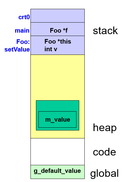
4 major memory segments
|
||||
|
||||
- Global: variables outside stack, heap
|
||||
- Code (a.k.a. text): the compiled program
|
||||
- Heap: dynamically allocated variables
|
||||
- Stack: parameters, automatic and temporary variables (all the variables that are declared inside a function, managed by the compiler, so must be fixed size)
|
||||
- _For the dynamically allocated variables, they will be allocated in the heap segment, but the pointer (fixed size) to them will be stored in the stack segment._
|
||||
|
||||
Key differences from Java
|
||||
|
||||
- Destructors of automatic variables called when stack frame where declared pops
|
||||
- No garbage collection: program must explicitly free dynamic memory
|
||||
|
||||
Heap and stack use varies dynamically
|
||||
|
||||
Code and global use is fixed
|
||||
|
||||
Code segment is "read-only"
|
||||
|
||||
```cpp
|
||||
int g_default_value = 1;
|
||||
|
||||
int main (int argc, char **argv) {
|
||||
Foo *f = new Foo;
|
||||
|
||||
f->setValue(g_default_value);
|
||||
|
||||
delete f; // programmer must explicitly free dynamic memory
|
||||
|
||||
return 0;
|
||||
}
|
||||
|
||||
void Foo::setValue(int v) {
|
||||
this->m_value = v;
|
||||
}
|
||||
```
|
||||
|
||||
|
||||
|
||||
### Memory, Lifetimes, and Scopes
|
||||
|
||||
Temporary variables
|
||||
|
||||
- Are scoped to an expression, e.g., `a = b + 3 * c;`
|
||||
|
||||
Automatic (stack) variables
|
||||
|
||||
- Are scoped to the duration of the function in which they are declared
|
||||
|
||||
Dynamically allocated variables
|
||||
|
||||
- Are scoped from explicit creation (new) to explicit destruction (delete)
|
||||
|
||||
Global variables
|
||||
|
||||
- Are scoped to the entire lifetime of the program
|
||||
- Includes static class and namespace members
|
||||
- May still have initialization ordering issues
|
||||
|
||||
Member variables
|
||||
|
||||
- Are scoped to the lifetime of the object within which they reside
|
||||
- Depends on whether object is temporary, automatic, dynamic, or global
|
||||
|
||||
**Lifetime of a pointer/reference can differ from the lifetime of the location to which it points/refers**
|
||||
|
||||
## Direct Dynamic Memory Allocation and Deallocation
|
||||
|
||||
```cpp
|
||||
#include <iostream>
|
||||
using namespace std;
|
||||
int main (int, char *[]) {
|
||||
int * i = new int; // any of these can throw bad_alloc
|
||||
int * j = new int(3);
|
||||
int * k = new int[*j];
|
||||
int * l = new int[*j];
|
||||
for (int m = 0; m < *j; ++m) { // fill the array with loop
|
||||
l[m] = m;
|
||||
}
|
||||
delete i; // call int destructor
|
||||
delete j; // single destructor call
|
||||
delete [] k; // call int destructor for each element
|
||||
delete [] l;
|
||||
return 0;
|
||||
}
|
||||
```
|
||||
|
||||
## Issues with direct memory management
|
||||
|
||||
### A Basic Issue: Multiple Aliasing
|
||||
|
||||
```cpp
|
||||
int main (int argc, char **argv) {
|
||||
Foo f;
|
||||
Foo *p = &f;
|
||||
Foo &r = f;
|
||||
delete p;
|
||||
return 0;
|
||||
}
|
||||
```
|
||||
|
||||
Multiple aliases for same object
|
||||
|
||||
- `f` is a simple alias, the object itself
|
||||
- `p` is a variable holding a pointer
|
||||
- `r` is a variable holding a reference
|
||||
|
||||
What happens when we call delete on p?
|
||||
|
||||
- Destroy a stack variable (may get a bus error there if we’re lucky)
|
||||
- If not, we may crash in destructor of f at function exit
|
||||
- Or worse, a local stack corruption that may lead to problems later
|
||||
|
||||
Problem: object destroyed but another alias to it was then used (**dangling pointer issue**)
|
||||
|
||||
### Memory Lifetime Errors
|
||||
|
||||
```cpp
|
||||
Foo *bad() {
|
||||
Foo f;
|
||||
return &f; // return address of local variable, f is destroyed after function returns
|
||||
}
|
||||
|
||||
Foo &alsoBad() {
|
||||
Foo f;
|
||||
return f; // return reference to local variable, f is destroyed after function returns
|
||||
}
|
||||
|
||||
Foo mediocre() {
|
||||
Foo f;
|
||||
return f; // return copy of local variable, f is destroyed after function returns, danger when f is a large object
|
||||
}
|
||||
|
||||
Foo * good() {
|
||||
Foo *f = new Foo;
|
||||
return f; // return pointer to local variable, with new we can return a pointer to a dynamically allocated object, but we must remember to delete it later
|
||||
}
|
||||
|
||||
int main() {
|
||||
Foo *f = &mediocre(); // f is a pointer to a temporary object, which is destroyed after function returns, f is invalid after function returns
|
||||
cout << good()->value() << endl; // good() returns a pointer to a dynamically allocated object, but we did not store the pointer, so it will be lost after function returns, making it impossible to delete it later.
|
||||
return 0;
|
||||
}
|
||||
```
|
||||
|
||||
Automatic variables
|
||||
|
||||
- Are destroyed on function return
|
||||
- But in bad, we return a pointer to a variable that no longer exists
|
||||
- Reference from also_bad similar
|
||||
- Like an un-initialized pointer
|
||||
|
||||
What if we returned a copy?
|
||||
|
||||
- Ok, we avoid the bad pointer, and end up with an actual object
|
||||
- But we do twice the work (why?)
|
||||
- And, it’s a temporary variable (more on this next)
|
||||
|
||||
We really want dynamic allocation here
|
||||
|
||||
Dynamically allocated variables
|
||||
|
||||
- Are not garbage collected
|
||||
- But are lost if no one refers to them: called a "**memory leak**"
|
||||
|
||||
Temporary variables
|
||||
|
||||
- Are destroyed at end of statement
|
||||
- Similar to problems w/ automatics
|
||||
|
||||
Can you spot 2 problems?
|
||||
|
||||
- One with a temporary variable
|
||||
- One with dynamic allocation
|
||||
|
||||
### Double Deletion Errors
|
||||
|
||||
```cpp
|
||||
int main (int argc, char **argv) {
|
||||
Foo *f = new Foo;
|
||||
delete f;
|
||||
// ... do other stuff
|
||||
delete f; // will throw an error because f is already deleted
|
||||
return 0;
|
||||
}
|
||||
```
|
||||
|
||||
What could be at this location?
|
||||
|
||||
- Another heap variable
|
||||
- Could corrupt heap
|
||||
|
||||
## Shared pointers and the RAII idiom
|
||||
|
||||
### A safer approach using smart pointers
|
||||
|
||||
C++11 provides two key dynamic allocation features
|
||||
|
||||
- `shared_ptr` : a reference counted pointer template to alias and manage objects allocated in dynamic memory (we’ll mostly use the shared_ptr smart pointer in this course)
|
||||
- `make_shared` : a function template that dynamically allocates and value initializes an object and then returns a shared pointer to it (hiding the object’s address, for safety)
|
||||
|
||||
C++11 provides 2 other smart pointers as well
|
||||
|
||||
- `unique_ptr` : a more complex but potentially very efficient way to transfer ownership of dynamic memory safely (implements C++11 “move semantics”)
|
||||
- `weak_ptr` : gives access to a resource that is guarded by a shared_ptr without increasing reference count (can be used to prevent memory leaks due to circular references)
|
||||
|
||||
### Resource Acquisition Is Initialization (RAII)
|
||||
|
||||
Also referred to as the "Guard Idiom"
|
||||
|
||||
- However, the term "RAII" is more widely used for C++
|
||||
|
||||
Relies on the fact that in C++ a stack object’s destructor is called when stack frame pops
|
||||
|
||||
Idea: we can use a stack object (usually a smart pointer) to hold the ownership of a heap object, or any other resource that requires explicit clean up
|
||||
|
||||
- Immediately initialize stack object with the allocated resource
|
||||
- De-allocate resource in the stack object’s destructor
|
||||
|
||||
### Example: Resource Acquisition Is Initialization (RAII)
|
||||
|
||||
```cpp
|
||||
shared_ptr<Foo> createAndInit() {
|
||||
shared_ptr<Foo> p =
|
||||
make_shared<Foo> ();
|
||||
init(p);// may throw exception
|
||||
return p;
|
||||
}
|
||||
|
||||
int run () {
|
||||
try {
|
||||
shared_ptr<Foo> spf =
|
||||
createAndInit();
|
||||
cout << “*spf is ” << *spf;
|
||||
} catch (...) {
|
||||
return -1
|
||||
}
|
||||
return 0;
|
||||
}
|
||||
```
|
||||
|
||||
RAII idiom example using shared_ptr
|
||||
|
||||
```cpp
|
||||
#include <memory>
|
||||
using namespace std;
|
||||
```
|
||||
|
||||
- `shared_ptr<X>` assumes and maintains ownership of aliased X
|
||||
- Can access the aliased X through it (*spf)
|
||||
- `shared_ptr<X>` destructor calls delete on address of owned X when it’s safe to do so (per reference counting idiom discussed next)
|
||||
- Combines well with other memory idioms
|
||||
|
||||
### Reference Counting
|
||||
|
||||
Basic Problem
|
||||
|
||||
- Resource sharing is often more efficient than copying
|
||||
- But it’s hard to tell when all are done using a resource
|
||||
- Must avoid early deletion
|
||||
- Must avoid leaks (non-deletion)
|
||||
|
||||
Solution Approach
|
||||
|
||||
- Share both the resource and a counter for references to it
|
||||
- Each new reference increments the counter
|
||||
- When a reference is done, it decrements the counter
|
||||
- If count drops to zero, also deletes resource and counter
|
||||
- "last one out shuts off the lights"
|
||||
|
||||
### Reference Counting Example
|
||||
|
||||
```cpp
|
||||
shared_ptr<Foo> createAndInit() {
|
||||
shared_ptr<Foo> p =
|
||||
make_shared<Foo> ();
|
||||
init(p);// may throw exception
|
||||
return p;
|
||||
}
|
||||
|
||||
int run () {
|
||||
try {
|
||||
shared_ptr<Foo> spf =
|
||||
createAndInit();
|
||||
shared_ptr<Foo> spf2 = spf;
|
||||
// object destroyed after
|
||||
// both spf and spf2 go away
|
||||
} catch (...) {
|
||||
return -1
|
||||
}
|
||||
return 0;
|
||||
}
|
||||
```
|
||||
|
||||
Again starts with RAII idiom via shared_ptr
|
||||
|
||||
- `spf` initially has sole ownership of aliased X
|
||||
- `spf.unique()` would return true
|
||||
- `spf.use_count` would return 1
|
||||
|
||||
`shared_ptr<X>` copy constructor increases count, and its destructor decreases count
|
||||
|
||||
`shared_ptr<X>` destructor calls delete on the pointer to the owned X when count drops to 0
|
||||
@@ -1,224 +0,0 @@
|
||||
# CSE332S Object-Oriented Programming in C++ (Lecture 14)
|
||||
|
||||
## Copy control
|
||||
|
||||
Copy control consists of 5 distinct operations
|
||||
|
||||
- A `copy constructor` initializes an object by duplicating the const l-value that was passed to it by reference
|
||||
- A `copy-assignment operator` (re)sets an object's value by duplicating the const l-value passed to it by reference
|
||||
- A `destructor` manages the destruction of an object
|
||||
- A `move constructor` initializes an object by transferring the implementation from the r-value reference passed to it (next lecture)
|
||||
- A `move-assignment operator` (re)sets an object's value by transferring the implementation from the r-value reference passed to it (next lecture)
|
||||
|
||||
Today we'll focus on the first 3 operations and will defer the others (introduced in C++11) until next time
|
||||
|
||||
- The others depend on the new C++11 `move semantics`
|
||||
|
||||
### Basic copy control operations
|
||||
|
||||
A copy constructor or copy-assignment operator takes a reference to a (usually const) instance of the class
|
||||
|
||||
- Copy constructor initializes a new object from it
|
||||
- Copy-assignment operator sets object's value from it
|
||||
- In either case, original the object is left unchanged (which differs from the move versions of these operations)
|
||||
- Destructor takes no arguments `~A()` (except implicit `this`)
|
||||
|
||||
Copy control operations for built-in types
|
||||
|
||||
- Copy construction and copy-assignment copy values
|
||||
- Destructor of built-in types does nothing (is a "no-op")
|
||||
|
||||
Compiler-synthesized copy control operations
|
||||
|
||||
- Just call that same operation on each member of the object
|
||||
- Uses defined/synthesized definition of that operation for user-defined types (see above for built-in types)
|
||||
|
||||
### Preventing or Allowing Basic Copy Control
|
||||
|
||||
Old (C++03) way to prevent compiler from generating a default constructor, copy constructor, destructor, or assignment operator was somewhat awkward
|
||||
|
||||
- Declare private, don't define, don't use within class
|
||||
- This works, but gives cryptic linker error if operation is used
|
||||
|
||||
New (C++11) way to prevent calls to any method
|
||||
|
||||
- End the declaration with `= delete` (and don't define)
|
||||
- Compiler will then give an intelligible error if a call is made
|
||||
|
||||
C++11 allows a constructor to call peer constructors
|
||||
|
||||
- Allows re-use of implementation (through delegation)
|
||||
- Object is fully constructed once any constructor finishes
|
||||
|
||||
C++11 lets you ask compiler to synthesize operations
|
||||
|
||||
- Explicitly, but only for basic copy control, default constructor
|
||||
- End the declaration with `= default` (and don't define) The compiler will then generate the operation or throw an error if it can't.
|
||||
|
||||
## Shallow vs Deep Copy
|
||||
|
||||
### Shallow Copy Construction
|
||||
|
||||
```cpp
|
||||
// just uses the array that's already in the other object
|
||||
IntArray::IntArray(const IntArray &a)
|
||||
:size_(a.size_),
|
||||
values_(a.values_) {
|
||||
// only memory address is copied, not the memory it points to
|
||||
}
|
||||
|
||||
int main(int argc, char * argv[]){
|
||||
IntArray arr = {0,1,2};
|
||||
IntArray arr2 = arr;
|
||||
return 0;
|
||||
}
|
||||
```
|
||||
|
||||
There are two ways to "copy"
|
||||
|
||||
- Shallow: re-aliases existing resources
|
||||
- E.g., by copying the address value from a pointer member variable
|
||||
- Deep: makes a complete and separate copy
|
||||
- I.e., by following pointers and deep copying what they alias
|
||||
|
||||
Version above shows shallow copy
|
||||
|
||||
- Efficient but may be risky (why?) The destructor will delete the memory that the other object is pointing to.
|
||||
- Usually want no-op destructor, aliasing via `shared_ptr` or a boolean value to check if the object is the original memory allocator for the resource.
|
||||
|
||||
### Deep Copy Construction
|
||||
|
||||
```cpp
|
||||
IntArray::IntArray(const IntArray &a)
|
||||
:size_(0), values_(nullptr) {
|
||||
|
||||
if (a.size_ > 0) {
|
||||
// new may throw bad_alloc,
|
||||
// set size_ after it succeeds
|
||||
values_ = new int[a.size_];
|
||||
size_ = a.size_;
|
||||
|
||||
// could use memcpy instead
|
||||
for (size_t i = 0;
|
||||
i < size_; ++i) {
|
||||
values_[i] = a.values_[i];
|
||||
}
|
||||
}
|
||||
}
|
||||
int main(int argc, char * argv[]){
|
||||
IntArray arr = {0,1,2};
|
||||
IntArray arr2 = arr;
|
||||
return 0;
|
||||
}
|
||||
|
||||
```
|
||||
|
||||
This code shows deep copy
|
||||
|
||||
- Safe: no shared aliasing, exception aware initialization
|
||||
- But may not be as efficient as shallow copy in many cases
|
||||
|
||||
Note trade-offs with arrays
|
||||
|
||||
- Allocate memory once
|
||||
- More efficient than multiple calls to new (heap search)
|
||||
- Constructor and assignment called on each array element
|
||||
- Less efficient than block copy
|
||||
- E.g., using `memcpy()`
|
||||
- But sometimes necessary
|
||||
- i.e., constructors, destructors establish needed invariants
|
||||
|
||||
Each object is responsible for its own resources.
|
||||
|
||||
## Swap Trick for Copy-Assignment
|
||||
|
||||
The swap trick is a way to implement the copy-assignment operator, given that the `size_` and `values_` members are already defined in constructor.
|
||||
|
||||
```cpp
|
||||
class Array {
|
||||
public:
|
||||
Array(unsigned int) ; // assume constructor allocates memory
|
||||
Array(const Array &); // assume copy constructor makes a deep copy
|
||||
~Array(); // assume destructor calls delete on values_
|
||||
Array & operator=(const Array &a);
|
||||
private:
|
||||
size_t size_;
|
||||
int * values_;
|
||||
};
|
||||
|
||||
Array & Array::operator=(const Array &a) { // return ref lets us chain
|
||||
if (&a != this) { // note test for self-assignment (safe, efficient)
|
||||
Array temp(a); // copy constructor makes deep copy of a
|
||||
swap(temp.size_, size_); // note unqualified calls to swap
|
||||
swap(temp.values_, values_); // (do user-defined or std::swap)
|
||||
}
|
||||
return *this; // previous *values_ cleaned up by temp's destructor, which is the member variable of the current object
|
||||
}
|
||||
|
||||
int main(int argc, char * argv[]){
|
||||
IntArray arr = {0,1,2};
|
||||
IntArray arr2 = {3,4,5};
|
||||
arr2 = arr;
|
||||
return 0;
|
||||
}
|
||||
|
||||
```
|
||||
|
||||
## Review: Construction/destruction order with inheritance, copy control with inheritance
|
||||
|
||||
### Constructor and Destructor are Inverses
|
||||
|
||||
```cpp
|
||||
IntArray::IntArray(unsigned int u)
|
||||
: size_(0), values_(nullptr) {
|
||||
// exception safe semantics
|
||||
values_ = new int [u];
|
||||
size_ = u;
|
||||
}
|
||||
|
||||
IntArray::~IntArray() {
|
||||
|
||||
// deallocates heap memory
|
||||
// that values_ points to,
|
||||
// so it's not leaked:
|
||||
// with deep copy, object
|
||||
// owns the memory
|
||||
delete [] values_;
|
||||
|
||||
// the size_ and values_
|
||||
// member variables are
|
||||
// themselves destroyed
|
||||
// after destructor body
|
||||
}
|
||||
```
|
||||
Constructors initialize
|
||||
|
||||
- At the start of each object's lifetime
|
||||
- Implicitly called when object is created
|
||||
|
||||
Destructors clean up
|
||||
|
||||
- Implicitly called when an object is destroyed
|
||||
- E.g., when stack frame where it was declared goes out of scope
|
||||
- E.g., when its address is passed to delete
|
||||
- E.g., when another object of which it is a member is being destroyed
|
||||
|
||||
### More on Initialization and Destruction
|
||||
|
||||
Initialization follows a well defined order
|
||||
|
||||
- Base class constructor is called
|
||||
- That constructor recursively follows this order, too
|
||||
- Member constructors are called
|
||||
- In order members were declared
|
||||
- Good style to list in that order (a good compiler may warn if not)
|
||||
- Constructor body is run
|
||||
|
||||
Destruction occurs in the reverse order
|
||||
|
||||
- Destructor body is run, then member destructors, then base class destructor (which recursively follows reverse order)
|
||||
|
||||
**Make destructor virtual if members are virtual**
|
||||
|
||||
- Or if class is part of an inheritance hierarchy
|
||||
- Avoids “slicing”: ensures destruction starts at the most derived class destructor (not at some higher base class)
|
||||
@@ -1,148 +0,0 @@
|
||||
# CSE332S Object-Oriented Programming in C++ (Lecture 15)
|
||||
|
||||
## Move semantics introduction and motivation
|
||||
|
||||
Review: copy control consists of 5 distinct operations
|
||||
|
||||
- A `copy constructor` initializes an object by duplicating the const l-value that was passed to it by reference
|
||||
- A `copy-assignment operator` (re)sets an object’s value by duplicating the const l-value passed to it by reference
|
||||
- A `destructor` manages the destruction of an object
|
||||
- A `move constructor` initializes an object by transferring the implementation from the r-value reference passed to it
|
||||
- A `move-assignment operator` (re)sets an object’s value by transferring the implementation from the r-value reference passed to it
|
||||
|
||||
Today we'll focus on the last 2 operations and other features (introduced in C++11) like r-value references
|
||||
I.e., features that support the new C++11 `move semantics`
|
||||
|
||||
### Motivation for move semantics
|
||||
|
||||
Copy construction and copy-assignment may be expensive due to time/memory for copying
|
||||
It would be more efficient to simply "take" the implementation from the passed object, if that's ok
|
||||
It's ok if the passed object won't be used afterward
|
||||
|
||||
- E.g., if it was passed by value and so is a temporary object
|
||||
- E.g., if a special r-value reference says it's ok to take from (as long as object remains in a state that's safe to destruct)
|
||||
|
||||
Note that some objects require move semantics
|
||||
|
||||
- I.e., types that don't allow copy construction/assignment
|
||||
- E.g., `unique_ptr`, `ifstream`, `thread`, etc.
|
||||
|
||||
New for C++11: r-value references and move function
|
||||
|
||||
- E.g., `int i; int &&rvri = std::move(i);`
|
||||
|
||||
### Synthesized move operations
|
||||
|
||||
Compiler will only synthesize a move operation if
|
||||
|
||||
- Class does not declare any copy control operations, and
|
||||
- Every non-static data member of the class can be moved
|
||||
|
||||
Members of built-in types can be moved
|
||||
|
||||
- E.g., by `std::move` etc.
|
||||
|
||||
User-defined types that have synthesized/defined version of the specific move operation can be moved
|
||||
L-values are always copied, r-values can be moved
|
||||
|
||||
- If there is no move constructor, r-values only can be copied
|
||||
|
||||
Can ask for a move operation to be synthesized
|
||||
|
||||
- I.e., by using `= default`
|
||||
- But if cannot move all members, synthesized as `= delete`
|
||||
|
||||
## Move constructor and assignment operator examples, more details on inheritance
|
||||
|
||||
### R-values, L-values, and Reference to Either
|
||||
|
||||
A variable is an l-value (has a location)
|
||||
|
||||
- E.g., `int i = 7;`
|
||||
|
||||
Can take a regular (l-value) reference to it
|
||||
|
||||
- E.g., `int & lvri = i;`
|
||||
|
||||
An expression is an r-value
|
||||
|
||||
- E.g., `i * 42`
|
||||
|
||||
Can only take an r-value reference to it (note syntax)
|
||||
|
||||
- E.g., `int && rvriexp = i * 42;`
|
||||
|
||||
Can only get r-value reference to l-value via move
|
||||
|
||||
- E.g., `int && rvri = std::move(i);`
|
||||
- Promises that i won’t be used for anything afterward
|
||||
- Also, must be safe to destroy i (could be stack/heap/global)
|
||||
|
||||
### Move Constructors
|
||||
|
||||
```cpp
|
||||
// takes implementation from a
|
||||
IntArray::IntArray(IntArray &&a)
|
||||
: size_(a.size_),
|
||||
values_(a.values_) {
|
||||
|
||||
// make a safe to destroy
|
||||
a.values_ = nullptr;
|
||||
a.size_ = 0;
|
||||
}
|
||||
```
|
||||
|
||||
Note r-value reference
|
||||
|
||||
- Says it's safe to take a's implementation from it
|
||||
- Promises only subsequent operation will be destruction
|
||||
|
||||
Note constructor design
|
||||
|
||||
- A lot like shallow copy constructor's implementation
|
||||
- Except, zeroes out state of `a`
|
||||
- No sharing, current object owns the implementation
|
||||
- Object `a` is now safe to destroy (but is not safe to do anything else with afterward)
|
||||
|
||||
### Move Assignment Operator
|
||||
|
||||
No allocation, so no exceptions to worry about
|
||||
|
||||
- Simply free existing implementation (delete `values_`)
|
||||
- Then copy over size and pointer values from `a`
|
||||
- Then zero out size and pointer in `a`
|
||||
|
||||
This leaves assignment complete, `a` safe to destroy
|
||||
|
||||
- Implementation is transferred from `a` to current object
|
||||
|
||||
```cpp
|
||||
Array & Array::operator=(Array &&a) { // Note r-value reference
|
||||
if (&a != this) { // still test for self-assignment
|
||||
delete [] values_; // safe to free first (if not self-assigning)
|
||||
size_ = a. size_; // take a’s size value
|
||||
values_ = a.values_; // take a’s pointer value
|
||||
a.size_ = 0; // zero out a’s size
|
||||
a.values_ = nullptr; // zero out a’s pointer (now safe to destroy)
|
||||
}
|
||||
return *this;
|
||||
}
|
||||
```
|
||||
|
||||
### Move Semantics and Inheritance
|
||||
|
||||
Base classes should declare/define move operations
|
||||
|
||||
- If it makes sense to do so at all
|
||||
- Derived classes then can focus on moving their members
|
||||
- E.g., calling `Base::operator=` from `Derived::operator=`
|
||||
|
||||
Containers further complicate these issues
|
||||
|
||||
- Containers hold their elements by value
|
||||
- Risks slicing, other inheritance and copy control problems
|
||||
|
||||
So, put (smart) pointers, not objects, into containers
|
||||
|
||||
- Access is polymorphic if destructors, other methods virtual
|
||||
- Smart pointers may help reduce need for copy control operations, or at least simplify cases where needed
|
||||
@@ -1,200 +0,0 @@
|
||||
# CSE332S Object-Oriented Programming in C++ (Lecture 16)
|
||||
|
||||
## Intro to OOP design and principles
|
||||
|
||||
### Review: Class Design
|
||||
|
||||
Designing a class to work well with the STL:
|
||||
|
||||
- What operators are required of our class?
|
||||
- `operator<` for ordered associative containers, `operator==` for unordered associative containers
|
||||
- `operator<<` and `operator>>` for interacting with iostreams
|
||||
- Algorithms require particular operators as well
|
||||
|
||||
Designing a class that manages dynamic resources:
|
||||
|
||||
- Must think about copy control
|
||||
- **Shallow copy** or **deep copy**?
|
||||
- When should the dynamic resources be cleaned up?
|
||||
- Move semantics for efficiency
|
||||
|
||||
### OOP Design: How do we combine objects to create complex software?
|
||||
|
||||
Goals - Software should be:
|
||||
|
||||
- Flexible
|
||||
- Extensible
|
||||
- Reusable
|
||||
|
||||
Today: 4 Principles of object-oriented programming
|
||||
|
||||
1. Encapsulation
|
||||
2. Abstraction
|
||||
3. Inheritance
|
||||
4. Polymorphism
|
||||
|
||||
#### Review: Client Code, interface vs. implementation
|
||||
|
||||
Today we will focus on a single class or family of classes related via a common
|
||||
base class and client code that interacts with it.
|
||||
|
||||
Next time: Combining objects to create more powerful and complex objects
|
||||
|
||||
**Client code**: code that has access to an object (via the object directly, a reference to the object, or a pointer/smart pointer to the object).
|
||||
|
||||
- Knows an object’s public interface only, not its implementation.
|
||||
|
||||
**Interface**: The set of all functions/operators (public member variables in C++ as well) a client can request of an object
|
||||
|
||||
**Implementation**: The definition of an object’s interface. State (member variables) and definitions of member functions/operators
|
||||
|
||||
#### Principle 1: Encapsulation
|
||||
|
||||
Data and behaviors are encapsulated together behind an interface
|
||||
|
||||
1. Member functions have direct access to the member variables of the object via “this”
|
||||
1. Benefit: Simplifies function calls (much smaller argument lists)
|
||||
|
||||
Proper encapsulation:
|
||||
|
||||
1. Data of a class remains internal (not enforced in C++)
|
||||
2. Client can only interact with the data of an object via its interface
|
||||
|
||||
**Benefit**:
|
||||
|
||||
(Flexible) Reduces impact of change - Easy to change how an object is stored
|
||||
without needing to modify client code that uses the object.
|
||||
|
||||
#### Principle 2: Abstraction
|
||||
|
||||
An object presents only the necessary interface to client code
|
||||
|
||||
1. Hides unnecessary implementation details from the client
|
||||
a. Member functions that client code does not need should be private or protected
|
||||
|
||||
We see abstraction everyday:
|
||||
|
||||
- TV
|
||||
- Cell phone
|
||||
- Coffee machine
|
||||
|
||||
Benefits:
|
||||
|
||||
1. Reduces code complexity, makes an object easier to use
|
||||
2. (Flexible) Reduces impact of change - internal implementation details can be
|
||||
modified without modification to client code
|
||||
|
||||
#### Principle 3: Inheritance (public inheritance in C++)
|
||||
|
||||
**"Implementation" inheritance - class inherits interface and implementation of
|
||||
its base class**
|
||||
|
||||
Benefits:
|
||||
|
||||
- Remove redundant code by placing it in a common base class.
|
||||
- (Reusable) Easily extend a class to add new functionality.
|
||||
|
||||
**"Interface" inheritance - inherit the interface of the base class only (abstract base class in C++, pure virtual functions)**
|
||||
|
||||
Benefits:
|
||||
|
||||
- Reduce dependencies between base/derived class
|
||||
- (Flexible, Extensible, Reusable) Program a client to depend on an interface rather than a specific implementation (more on this later)
|
||||
|
||||
#### One More Useful C++ Construct: Multiple Inheritance
|
||||
|
||||
C++ allows a class to inherit from more than one base class
|
||||
|
||||
```cpp
|
||||
class Bear: public ZooAnimal {/*...*/};
|
||||
class Panda: public Bear, public Endangered {/*...*/};
|
||||
```
|
||||
|
||||
Construction order - all base classes are constructed first:
|
||||
|
||||
- all base classes -> derived classes member variables -> constructor body
|
||||
|
||||
Destruction order - opposite of construction order:
|
||||
|
||||
- Destructor body -> derived classes member variables -> all base class
|
||||
destructors
|
||||
|
||||
**Rule of thumb**: When using multiple inheritance, a class should inherit
|
||||
implementation from a single base class only. Any number of interfaces may be
|
||||
inherited (this is enforced in Java)
|
||||
|
||||
#### Principle 4: Polymorphism
|
||||
|
||||
A single interface may have many different implementations (virtual functions and
|
||||
function overriding in C++)
|
||||
|
||||
Benefits:
|
||||
|
||||
1. Avoid nasty switch statements (function calls resolved dynamically)
|
||||
2. (Flexible) Allows the implementation of an interface to change at run-time
|
||||
|
||||
#### Program to an interface
|
||||
|
||||
Client should restrict variables to an interface only, not a specific implementation
|
||||
|
||||
- **Extensible, reusable**: New subclasses that define the interface can be created and used without modification to the client. Easy to add new functionality. Easy to reuse client.
|
||||
- **Reduce impact of change**: Decouples client from concrete classes it uses.
|
||||
- **Flexible**: The implementation of an interface used by the client can change at run-time.
|
||||
|
||||
In C++:
|
||||
|
||||
- Abstract base class using pure virtual functions to declare the interface
|
||||
- Implement the interface in subclasses via public inheritance
|
||||
- Client maintains reference or pointer to the base class
|
||||
- Calls through the reference or pointer are polymorphic
|
||||
|
||||
```cpp
|
||||
// declare printable interface
|
||||
class printable {
|
||||
public:
|
||||
virtual void print(ostream &o) = 0;
|
||||
};
|
||||
// derived classes defines printable
|
||||
// interface
|
||||
class smiley : public printable {
|
||||
public:
|
||||
virtual void print(ostream &o) {
|
||||
o << ":)" ;
|
||||
};
|
||||
};
|
||||
class frown : public printable {
|
||||
public:
|
||||
virtual void print(ostream &o) {
|
||||
o << ":(";
|
||||
};
|
||||
};
|
||||
int main(int argc, char * argv[]) {
|
||||
smiley s; // s restricted to
|
||||
// a smiley object
|
||||
s.print();
|
||||
// p may point to an object
|
||||
// of any class that defines
|
||||
// the printable interface
|
||||
printable * p =
|
||||
generateOutput();
|
||||
// Client unaware of the
|
||||
// implementation of print()
|
||||
p->print();
|
||||
return 0;
|
||||
}
|
||||
```
|
||||
|
||||
Program to an interface
|
||||
Allows easily extensible designs: anything that defines the printable interface can
|
||||
be used with our client
|
||||
|
||||
```cpp
|
||||
class Book : public printable {
|
||||
vector<string> pages;
|
||||
public:
|
||||
virtual void print(ostream &o) {
|
||||
for(unsigned int page = 0; page < pages.size(); ++page){
|
||||
o << "page: " << page << endl;
|
||||
o << pages[i] << endl;
|
||||
};
|
||||
};
|
||||
@@ -1,147 +0,0 @@
|
||||
# CSE332S Object-Oriented Programming in C++ (Lecture 17)
|
||||
|
||||
## Object Oriented Programming Building Blocks
|
||||
|
||||
OOP Building Blocks for Extensible, Flexible, and Reusable Code
|
||||
|
||||
Today: Techniques Commonly Used in Design Patterns
|
||||
|
||||
- **Program to an interface** (last time)
|
||||
- **Object composition and request forwarding** (today)
|
||||
- Composition vs. inheritance
|
||||
- **Run-time relationships between objects** (today)
|
||||
- Aggregate vs. acquaintance
|
||||
- **Delegation** (later...)
|
||||
|
||||
Next Time: Design Patterns
|
||||
|
||||
Describe the core of a repeatable solution to common design problems.
|
||||
|
||||
### Code Reuse: Two Ways to Reuse a Class
|
||||
|
||||
#### Inheritance
|
||||
|
||||
Code reuse by inheriting the implementation of a base class.
|
||||
|
||||
- **Pros:**
|
||||
- Inheritance relationships defined at compile-time - simple to understand.
|
||||
- **Cons:**
|
||||
- Subclass often inherits some implementation from superclass - derived class now depends on its base class implementation, leading to less flexible code.
|
||||
|
||||
#### Composition
|
||||
|
||||
Assemble multiple objects together to create new complex functionality, forward requests to the responsible assembled object.
|
||||
|
||||
- **Pros:**
|
||||
- Allows flexibility at run-time, composite objects often constructed dynamically by obtaining references/pointers to other objects (dependency injection).
|
||||
- Objects known only through their interface - increased flexibility, reduced impact of change.
|
||||
- **Cons:**
|
||||
- Code can be more difficult to understand, how objects interact may change dynamically.
|
||||
|
||||
### Example: Our First Design Pattern (Adapter Pattern)
|
||||
|
||||
**Problem:** We are given a class that we cannot modify for some reason - it provides functionality we need, but defines an interface that does not match our program (client code).
|
||||
|
||||
**Solution:** Create an adapter class, adapter declares the interface needed by our program, defines it by forwarding requests to the unmodifiable object.
|
||||
|
||||
Two ways to do this:
|
||||
|
||||
```cpp
|
||||
class unmodifiable {
|
||||
public:
|
||||
int func(); // does something useful, but doesn’t match the interface required by the client code
|
||||
};
|
||||
```
|
||||
|
||||
1. **Inheritance**
|
||||
|
||||
```cpp
|
||||
// Using inheritance:
|
||||
class adapter : protected unmodifiable {
|
||||
// open the access to the protected member func() for derived class
|
||||
public:
|
||||
int myFunc() {
|
||||
return func(); // forward request to encapsulated object
|
||||
}
|
||||
};
|
||||
```
|
||||
|
||||
2. **Composition**
|
||||
|
||||
```cpp
|
||||
class adapterComp {
|
||||
unmodifiable var;
|
||||
public:
|
||||
int myFunc() {
|
||||
return var.func();
|
||||
}
|
||||
};
|
||||
```
|
||||
|
||||
### Thinking About and Describing Run-time Relationships
|
||||
|
||||
Typically, composition is favored over inheritance! Object composition with programming to an interface allows relationships/interactions between objects to vary at run-time.
|
||||
|
||||
- **Aggregate:** Object is part of another. Its lifetime is the same as the object it is contained in. (similar to base class and derived class relationship)
|
||||
- **Acquaintance:** Objects know of each other, but are not responsible for each other. Lifetimes may be different.
|
||||
|
||||
```cpp
|
||||
// declare Printable Interface
|
||||
// declare printable interface
|
||||
class printable {
|
||||
public:
|
||||
virtual void print(ostream &o) = 0;
|
||||
};
|
||||
// derived classes defines printable
|
||||
// interface
|
||||
class smiley : public printable {
|
||||
public:
|
||||
virtual void print(ostream &o) {
|
||||
o << ":)";
|
||||
};
|
||||
};
|
||||
// second derived class defines
|
||||
// printable interface
|
||||
class frown : public printable {
|
||||
public:
|
||||
virtual void print(ostream &o) {o << ":(";
|
||||
};
|
||||
};
|
||||
```
|
||||
|
||||
1. **Aggregate**
|
||||
|
||||
```cpp
|
||||
// implementation 1:
|
||||
// Aggregate relationship
|
||||
class emojis {
|
||||
printable * happy;
|
||||
printable * sad;
|
||||
public:
|
||||
emojis() {
|
||||
happy = new smiley();
|
||||
sad = new frown();
|
||||
};
|
||||
~emojis() {
|
||||
delete happy;
|
||||
delete sad;
|
||||
};
|
||||
};
|
||||
```
|
||||
|
||||
2. **Acquaintance**
|
||||
|
||||
```cpp
|
||||
// implementation 2:
|
||||
// Acquaintances only
|
||||
class emojis {
|
||||
printable * happy;
|
||||
printable * sad;
|
||||
public:
|
||||
emojis();
|
||||
~emojis();
|
||||
// dependency injection
|
||||
void setHappy(printable *);
|
||||
void setSad(printable *);
|
||||
};
|
||||
```
|
||||
@@ -1,256 +0,0 @@
|
||||
# CSE332S Object-Oriented Programming in C++ (Lecture 2)
|
||||
|
||||
Today we'll talk generally about C++ development (plus a few platform specifics):
|
||||
|
||||
- We'll develop, submit, and grade code in Windows
|
||||
- It's also helpful to become familiar with Linux
|
||||
- E.g., on shell.cec.wustl.edu
|
||||
- For example, running code through two different compilers can catch a lot more "easy to make" errors
|
||||
|
||||
Extra credit on Lab 1: compile the cpp program in Linux.
|
||||
|
||||
## Writing C++
|
||||
|
||||
Makefile ASCII text
|
||||
|
||||
C++ course files, ASCII text, end it with .cpp
|
||||
|
||||
C++ header files, ASCII text, end it with .h
|
||||
|
||||
readme, ASCII text (show what program does)
|
||||
|
||||
## Parts of a C++ Program
|
||||
|
||||
### Declarations
|
||||
|
||||
data types, function signatures, class declarations
|
||||
|
||||
- This allows the compiler to check for type safety, correct syntax, and other errors
|
||||
- Usually kept in header files (e.g., .h)
|
||||
- Included as needed by other files (to make compiler happy)
|
||||
|
||||
```cpp
|
||||
// my_class.h
|
||||
class Simple {
|
||||
public:
|
||||
Simple (int i);
|
||||
void print_i();
|
||||
private:
|
||||
int i_;
|
||||
}
|
||||
|
||||
typedef unsigned int UNIT32;
|
||||
|
||||
int usage (char * program_name);
|
||||
|
||||
struct Point2D {
|
||||
double x_;
|
||||
double y_;
|
||||
};
|
||||
```
|
||||
|
||||
### Definitions
|
||||
|
||||
Static variables initialization, function implementation
|
||||
|
||||
- The part that turns into an executable program
|
||||
- Usually kept in source files (e.g., .cpp)
|
||||
|
||||
```cpp
|
||||
// my_class.cpp
|
||||
#include "my_class.h"
|
||||
|
||||
Simple::Simple (int i) : i_(i) {}
|
||||
|
||||
void Simple::print_i() {
|
||||
std::cout << i_ << std::endl;
|
||||
}
|
||||
```
|
||||
|
||||
### Directives
|
||||
|
||||
tell complier or preprocessor what to do
|
||||
|
||||
more on this later
|
||||
|
||||
## A Very Simple C++ Program
|
||||
|
||||
```cpp
|
||||
#include <iostream> // precompiler directive
|
||||
|
||||
using namespace std; // compiler directive
|
||||
|
||||
// definition of main function
|
||||
|
||||
int main(int, char *[]) {
|
||||
cout << "Hello, World!" << endl;
|
||||
return 0;
|
||||
}
|
||||
```
|
||||
|
||||
### What is `#include <iostream>`?
|
||||
|
||||
- `#include` tells the precompiler to include a file
|
||||
- Usually, we include header files that:
|
||||
- Contain declarations of structs, classes, functions
|
||||
- Sometimes contain template _definitions_ (template not included in this course)
|
||||
- Implementation varies from compiler to compiler (advanced topic covered later)
|
||||
- `<iostream>` is the C++ standard header file for input/output streams
|
||||
|
||||
### What is `using namespace std;`?
|
||||
|
||||
- The `using` directive tells the compiler to include code from libraries that have separate namespaces
|
||||
- Similar idea to "packages" in other languages
|
||||
- C++ provides a namespace for its standard library
|
||||
- Called the "standard namespace" (written as `std`)
|
||||
- Contains `cout`, `cin`, `cerr` standard iostreams, and much more
|
||||
- Namespaces reduce collisions between symbols
|
||||
- Rely on the `::` scoping operator to match symbols to them
|
||||
- If another library with namespace `mylib` defined `cout` we could say `std::cout` vs. `mylib::cout`
|
||||
- Can also apply `using` more selectively:
|
||||
- E.g., just `using std::cout`
|
||||
|
||||
### What is `int main(int, char *[]) { ... }`?
|
||||
|
||||
- Defines the main function of any C++ program, it is the entry point of the program
|
||||
|
||||
- Who calls main?
|
||||
- The runtime environment, specifically a function often called something like `crt0` or `crtexe`
|
||||
|
||||
- What about the stuff in parentheses?
|
||||
- A list of types of the input arguments to function `main`
|
||||
- With the function name, makes up its signature
|
||||
- Since this version of `main` ignores any inputs, we leave off names of the input variables, and only give their types
|
||||
|
||||
- What about the stuff in braces?
|
||||
- It's the body of function `main`, its definition
|
||||
|
||||
### What is `cout << "Hello, World!" << endl;`?
|
||||
|
||||
- Uses the standard output iostream, named `cout`
|
||||
- For standard input, use `cin`
|
||||
- For standard error, use `cerr`
|
||||
- `<<` is an operator for inserting into the stream
|
||||
- A member operator of the `ostream` class
|
||||
- Returns a reference to stream on which it's called
|
||||
- Can be applied repeatedly to references left-to-right
|
||||
- `"hello, world!"` is a C-style string
|
||||
- A 14-position character array terminated by `'\0'`
|
||||
- `endl` is an iostream manipulator
|
||||
- Ends the line by inserting end-of-line character(s)
|
||||
- Also flushes the stream
|
||||
|
||||
### What about `return 0;`?
|
||||
|
||||
- The `main` function must return an integer value
|
||||
- By convention:
|
||||
- Return `0` to indicate successful execution
|
||||
- Return non-zero value to indicate failure
|
||||
- The program should exit gracefully through `main`'s return
|
||||
- Other ways the program can terminate abnormally:
|
||||
- Uncaught exceptions propagating out of `main`
|
||||
- Division by zero
|
||||
- Dereferencing null pointers
|
||||
- Accessing memory not owned by the program
|
||||
- Array index out of bounds
|
||||
- Dereferencing invalid/"stray" pointers
|
||||
|
||||
## A slightly more complex program
|
||||
|
||||
```cpp
|
||||
#include <iostream>
|
||||
|
||||
using namespace std;
|
||||
|
||||
int main(int argc, char *argv[]) {
|
||||
for (int i = 0; i < argc; i++) {
|
||||
cout << argv[i] << endl;
|
||||
}
|
||||
return 0;
|
||||
}
|
||||
```
|
||||
|
||||
### `int argc, char *argv[]`
|
||||
|
||||
- A way to affect the program's behavior
|
||||
- Carry parameters with which program was called
|
||||
- Passed as parameters to main from crt0
|
||||
- Passed by value (we'll discuss what that means)
|
||||
|
||||
`argc`:
|
||||
|
||||
- An integer with the number of parameters (>=1)
|
||||
|
||||
`argv`:
|
||||
|
||||
- An array of pointers to C-style character strings
|
||||
- **Its array-length is the value stored in `argc`**
|
||||
- The name of the program is kept in `argv[0]`
|
||||
|
||||
### What is `for (int i = 0; i < argc; i++) { ... }`?
|
||||
|
||||
Standard C++ for loop syntax:
|
||||
|
||||
- Consists of 3 parts:
|
||||
1. Initialization statement (executed once at start)
|
||||
2. Test expression (checked before each iteration)
|
||||
3. Increment expression (executed after each iteration)
|
||||
|
||||
Let's break down each part:
|
||||
|
||||
`int i = 0`:
|
||||
|
||||
- Declares integer variable `i` (scoped to the loop)
|
||||
- Initializes `i` to 0 (initialization, not assignment)
|
||||
|
||||
`i < argc`:
|
||||
|
||||
- Tests if we're within array bounds
|
||||
- Critical for memory safety - accessing outside array can crash program
|
||||
|
||||
`++i`:
|
||||
|
||||
- Increments array position counter
|
||||
- Uses prefix increment operator
|
||||
|
||||
## Lifecycle of a C++ Program
|
||||
|
||||
Start from the makefile
|
||||
|
||||
- The makefile is a text file that tells the compiler how to build the program, it activates the 'make' utility to build the program
|
||||
- The make file turnin/checkin to the WebCAT E-mail
|
||||
- The makefile complies the gcc compiler to compile the cpp file
|
||||
- The makefile links the object files to create the executable file
|
||||
|
||||
The cpp file
|
||||
|
||||
- The cpp file is a text file that contains the source code of the program
|
||||
- The cpp file is compiled into an object file by the gcc compiler to combined with the link produced by the makefile with the runtime/util library
|
||||
|
||||
Finally, the object file is linked with the runtime/util library to create the executable program and ready to debug with Eclipse or Visual Studio.
|
||||
|
||||
## Development Environment Studio
|
||||
|
||||
### Course Format
|
||||
|
||||
- We'll follow a similar format most days in the course:
|
||||
- Around 30 minutes of lecture and discussion
|
||||
- Then about 60 minutes of studio time
|
||||
- Except for:
|
||||
- Open studio/lab days
|
||||
- Reviews before the midterm and final
|
||||
- The day of the midterm itself
|
||||
|
||||
### Studio Guidelines
|
||||
|
||||
- Work in groups of 2 or 3
|
||||
- Exercises are posted on the course web page
|
||||
- Record your answers and email them to the course account
|
||||
- Instructors will circulate to answer questions
|
||||
|
||||
### Purpose of Studios
|
||||
|
||||
- Develop skills and understanding
|
||||
- Explore ideas you can use for labs
|
||||
- Prepare for exams which test studio material
|
||||
- Encouraged to try variations beyond exercises
|
||||
@@ -1,308 +0,0 @@
|
||||
# CSE332S Object-Oriented Programming in C++ (Lecture 3)
|
||||
|
||||
## C++ basic data types
|
||||
|
||||
- int, long, short, char (signed, integer arithmetic)
|
||||
- char is only 1 byte for all platforms
|
||||
- other types are platform dependent
|
||||
- can determine the size of the type by using `sizeof()`, `<climits> INT_MAX`
|
||||
- float, double (floating point arithmetic)
|
||||
- more expensive in space and time
|
||||
- useful when you need to describe continuous quantities
|
||||
- bool (boolean logic)
|
||||
|
||||
### User-defined types
|
||||
|
||||
- (unscoped or scoped) enum
|
||||
- maps a sequence of integer values to named constants
|
||||
- function and operators
|
||||
- function is a named sequence of statements, for example `int main()`
|
||||
- struct and class
|
||||
- similar to abstractions in cpp, extend C struct
|
||||
|
||||
### struct and class
|
||||
|
||||
- struct is public by default
|
||||
- class is private by default
|
||||
- both can have
|
||||
- member variables
|
||||
- member functions
|
||||
- constructors
|
||||
- destructors
|
||||
- common practice:
|
||||
- use struct for simple data structures
|
||||
- use class for more complex data structures with non-trivial functionality
|
||||
|
||||
```cpp
|
||||
struct My_Data{
|
||||
My_Data(int x, int y): x_(x), y_(y) {}
|
||||
int x_;
|
||||
int y_;
|
||||
};
|
||||
```
|
||||
|
||||
```cpp
|
||||
class My_Data{
|
||||
public:
|
||||
My_Object(int x, int y): x_(x), y_(y) {}
|
||||
~My_Object(){}
|
||||
private:
|
||||
int x_;
|
||||
int y_;
|
||||
};
|
||||
```
|
||||
|
||||
### More about native and user-defined types
|
||||
|
||||
- Pointer
|
||||
- raw memory address of an object
|
||||
- its type constrains what types it can point to
|
||||
- can take on a value of 0 (null pointer)
|
||||
- Reference
|
||||
- alias for an existing object
|
||||
- its type constrains what types it can refer to
|
||||
- cannot take on a value of 0 (**always** refer to a valid object)
|
||||
- Mutable (default) vs. const types (read right to left)
|
||||
- `const int x;` is a read-only variable
|
||||
- `int j` is a read-write declaration
|
||||
|
||||
## Scopes
|
||||
|
||||
Each variable is associated with a scope, which is a region of the program where the variable is valid
|
||||
|
||||
- the entire program is a global scope
|
||||
- a namespace is a scope
|
||||
- member of a class is a scope
|
||||
- a function is a scope
|
||||
- a block is a scope
|
||||
|
||||
```cpp
|
||||
int g_x; // global scope
|
||||
namespace my_namespace{
|
||||
int n_x; // namespace scope
|
||||
}
|
||||
class My_Class{
|
||||
int c_x; // class scope
|
||||
int my_function(){
|
||||
int f_x; // function scope
|
||||
{
|
||||
int b_x; // block scope
|
||||
}
|
||||
return 0;
|
||||
}
|
||||
}
|
||||
```
|
||||
|
||||
A symbol is only visible within its scope
|
||||
|
||||
- helps hide unneeded details (abstraction)
|
||||
- helps avoid name collisions (encapsulation)
|
||||
|
||||
## Motivation for pointer and reference
|
||||
|
||||
We often need to _refer_ to an object, but don't want to copy it
|
||||
|
||||
There are two common ways to do this:
|
||||
|
||||
- Indirectly, via a pointer
|
||||
- This gives the address of the object
|
||||
- Requires the code to do extra work. eg, dereferencing
|
||||
- Like going to the address of the object
|
||||
- Directly, via a reference
|
||||
- Acts as an alias for the object
|
||||
- Code interacts with reference as if it were the object itself
|
||||
|
||||
## Pointer and reference syntax
|
||||
|
||||
### Pointer
|
||||
|
||||
A pointer is a variable that holds the address of an object
|
||||
|
||||
can be untyped. eg, `void *p;`
|
||||
|
||||
usually typed. eg, `int *p;` so that it can be checked by the compiler
|
||||
|
||||
If typed, the type constrains what it can point to, a int pointer can only point to an int. `int *p;`
|
||||
|
||||
A pointer can be null, eg, `int *p = nullptr;`
|
||||
|
||||
We can change to what it points to, eg, `p = &x;`
|
||||
|
||||
### Reference
|
||||
|
||||
A reference is an alias for an existing object, also holds the address of the object, but is only created on compile time.
|
||||
|
||||
Usually with nicer interface than pointers.
|
||||
|
||||
Must be typed, and its type constrains what types it can refer to. `int &r;`
|
||||
|
||||
Always refers to a valid object, so cannot be null. `int &r = nullptr;` is invalid.
|
||||
|
||||
Note: **reference cannot be reassigned to refer to a different object.**
|
||||
|
||||
|symbol|used in declaration|used in definition|
|
||||
|---|---|---|
|
||||
|unary `&`|reference, eg, `int &r;`|address-of, eg, `int &r = &x;`|
|
||||
|unary `*`|pointer, eg, `int *p;`|dereference, eg, `int *p = *q;`|
|
||||
|`->`|member access, eg, `p->x;`|member access via pointer, eg, `p->second;`|
|
||||
|`.`|member access, eg, `p.x;`|member access via reference, eg, `p.second;`|
|
||||
|
||||
## Aliasing via pointers and references
|
||||
|
||||
### Aliasing via reference
|
||||
|
||||
Example:
|
||||
|
||||
```cpp
|
||||
int main(int argc, char *argv[]){
|
||||
int i=0;
|
||||
int j=1;
|
||||
int &r = i;
|
||||
int &s = i;
|
||||
r = 8; // do not need to dereference r, just use it as an alias for i
|
||||
cout << "i: " << i << ", j: " << j << ", r: " << r << ", s: " << s << endl;
|
||||
// should print: i: 8, j: 1, r: 8, s: 8
|
||||
return 0;
|
||||
}
|
||||
```
|
||||
|
||||
### Aliasing via pointer
|
||||
|
||||
Example:
|
||||
|
||||
```cpp
|
||||
int main(int argc, char *argv[]){
|
||||
int i=0;
|
||||
int j=1;
|
||||
int *p = &i;
|
||||
int *q = &i;
|
||||
*q = 6; // need to dereference q to access the value of j
|
||||
cout << "i: " << i << ", j: " << j << ", p: " << *p << ", q: " << *q << endl;
|
||||
// should print: i: 6, j: 1, p: 6, q: 6
|
||||
return 0;
|
||||
}
|
||||
```
|
||||
|
||||
### Reference to Pointer
|
||||
|
||||
Example:
|
||||
|
||||
```cpp
|
||||
int main(int argc, char *argv[]){
|
||||
int j = 1;
|
||||
int &r = j; // r is a **reference** to j
|
||||
int *p = &r; // p is a **pointer** to the address of r, here & is the address-of operator, which returns the address of the object
|
||||
int * &t = p; // t is a **reference** to pointer p, here & is the reference operator, which returns the reference of the object.
|
||||
cout << "j: " << j << ", r: " << r << ", p: " << *p << ", t: " << *t << endl;
|
||||
// should print: j: 1, r: 1, p: 1, t: [address of p]
|
||||
return 0;
|
||||
}
|
||||
```
|
||||
|
||||
Notice that we cannot have a pointer to a reference. But we can have a reference to a pointer.
|
||||
|
||||
### Reference to Constant
|
||||
|
||||
Example:
|
||||
|
||||
```cpp
|
||||
int main(int argc, char *argv[]){
|
||||
const int i = 0;
|
||||
int j = 1;
|
||||
int &r = j; // r cannot refer to i, because i is a constant (if true, alter i through r should be valid)
|
||||
const int &s=i; // s can refer to i, because s is a constant reference (we don't reassign s)
|
||||
const int &t=j; // t can refer to j, because t is a constant reference (we don't reassign t)
|
||||
cout << "i: " << i << ", j: " << j << ", r: " << r << ", s: " << s << ", t: " << t << endl;
|
||||
// should print: i: 0, j: 1, r: 1, s: 0
|
||||
return 0;
|
||||
}
|
||||
```
|
||||
|
||||
Notice that we cannot have a non-constant reference to a constant object. But we can have a constant reference to a non-constant object.
|
||||
|
||||
### Pointer to Constant
|
||||
|
||||
Example:
|
||||
|
||||
```cpp
|
||||
int main(int argc, char *argv[]){
|
||||
const int i = 0;
|
||||
int j = 1;
|
||||
int k = 2;
|
||||
|
||||
// pointer to int
|
||||
int *w = &j;
|
||||
|
||||
// const pointer to int
|
||||
int *const x = &j;
|
||||
|
||||
// pointer to const int
|
||||
const int *y = &i;
|
||||
|
||||
// const pointer to const int, notice that we cannot change the value of the int that z is pointing to, in this case j **via pointer z**, nor the address that z is pointing to. But we can change the value of j via pointer w or j itself.
|
||||
const int *const z = &j;
|
||||
}
|
||||
```
|
||||
|
||||
- Read declaration from right to left, eg, `int *w = &j;` means `w` is a pointer to an `int` that is the address of `j`.
|
||||
- Make promises via the `const` keyword, two options:
|
||||
- `const int *p;` means `p` is a pointer to a constant `int`, so we cannot change the value of the `int` that `p` is pointing to, but we can change the address that `p` is pointing to.
|
||||
- `int *const p;` means `p` is a constant pointer to an `int`, so we cannot change the address that `p` is pointing to, but we can change the value of the `int` that `p` is pointing to.
|
||||
- A pointer to non-constant cannot point to a const variable.
|
||||
- neither `w = &i;` nor `x = &i;` is valid.
|
||||
- any of the pointer can points to `j`.
|
||||
|
||||
## Pass by value, pass by reference, and type inference
|
||||
|
||||
Example:
|
||||
|
||||
```cpp
|
||||
int main(int argc, char *argv[]){
|
||||
int h = -1;
|
||||
int i = 0;
|
||||
int j = 1;
|
||||
int k = 2;
|
||||
return func(h, i, j, &k);
|
||||
}
|
||||
|
||||
int func(int a, const int &b, int &c, int *d){
|
||||
++a; // [int] pass by value, a is a copy of h, so a is not the same as h
|
||||
c = b; // [int &] pass by reference, c is an alias for j, the value of c is the same as the value of b (or i), but we cannot change the value of b (or i) through c (const int &b)
|
||||
*d = a; // [int *] pass by value, d is a pointer to k, so *d is the value of k, a is assigned to value of k.
|
||||
++d; // d is a pointer to k, but pass by value, so ++d doesn't change the value of k.
|
||||
return 0;
|
||||
}
|
||||
```
|
||||
|
||||
### More type declaration keywords
|
||||
|
||||
`typedef` keyword introduces a "type alias" for a type.
|
||||
|
||||
```cpp
|
||||
typedef Foo * Foo_ptr; // Foo_ptr is a type alias for Foo *
|
||||
|
||||
// the following two variables are of the same type
|
||||
Foo_ptr p1 = 0;
|
||||
Foo *p2 = 0;
|
||||
```
|
||||
|
||||
`auto` keyword allows the compiler to deduce the type of a variable from the initializer.
|
||||
|
||||
```cpp
|
||||
int x = 0; // x is of type int
|
||||
float y = 1.0; // y is of type float
|
||||
auto z = x + y; // z is of type float, with initialized value 1.0
|
||||
```
|
||||
|
||||
`decltype` keyword allows the compiler to deduce the type of a variable from the type of an expression.
|
||||
|
||||
```cpp
|
||||
int x = 0;
|
||||
double y = 0.0;
|
||||
float z = 0.0f;
|
||||
|
||||
decltype(x) a; // a is of type int, value is not initialized
|
||||
decltype(y) b; // b is of type double, value is not initialized
|
||||
decltype(z) c; // c is of type float, value is not initialized
|
||||
```
|
||||
|
||||
@@ -1,478 +0,0 @@
|
||||
# CSE332S Object-Oriented Programming in C++ (Lecture 4)
|
||||
|
||||
## Namespace details
|
||||
|
||||
### Motivation
|
||||
|
||||
Classes encapsulate behavior (methods) and state (member data) behind an interface.
|
||||
|
||||
Structs are similar, but with state accessible.
|
||||
|
||||
Classes and structs are used to specify self contained, cohesive abstractions.
|
||||
|
||||
- Can say what class/struct does in one sentence.
|
||||
|
||||
What if we want to describe more loosely related collections of state and behavior?
|
||||
|
||||
Could use a class or struct
|
||||
|
||||
- But that dilutes their design intent.
|
||||
|
||||
### Namespace
|
||||
|
||||
Cpp offers an appropriate scoping mechanism for **loosely related** aggregates: Namespaces.
|
||||
|
||||
- Good for large function collections.
|
||||
- E.g. a set of related algorithms and function objects
|
||||
- Good for general purpose collections
|
||||
- E.g. program utilities, performance statistics, etc.
|
||||
|
||||
Declarative region
|
||||
|
||||
- Where a variable/function can be used
|
||||
- From where declared to end of declarative region
|
||||
|
||||
### Namespace Properties
|
||||
|
||||
Declared/(re)opend with `namespace` keyword.
|
||||
|
||||
- `namespace name { ... }`
|
||||
- `namespace name = namespace existing_name { ... };`
|
||||
|
||||
Access members using scoping `operator::`
|
||||
|
||||
- `std::cout << "Hello, World!" << std::endl;`
|
||||
|
||||
Everything not declared in another namespace is in the global namespace.
|
||||
|
||||
Can nest namespace declarations
|
||||
|
||||
- `namespace outer { namespace inner { ... } }`
|
||||
|
||||
### Using Namespaces
|
||||
|
||||
The `using` keyword make elements visible.
|
||||
|
||||
- Only apples to the current scope.
|
||||
|
||||
Can add entire name space to the current scope
|
||||
|
||||
- `using namespace std;`
|
||||
- `cout << "Hello, World!" << endl;`
|
||||
|
||||
Can also declare unnamed namespaces
|
||||
|
||||
- Elements are visible after the declaration
|
||||
- `namespace { int i = 42; }` will make `i` visible in the current file.
|
||||
|
||||
## C-style vs. C++ strings
|
||||
|
||||
### C++ string class
|
||||
|
||||
```cpp
|
||||
#include <iostream>
|
||||
#include <string>
|
||||
|
||||
using namespace std;
|
||||
|
||||
int main (int argc, char *argv[]) {
|
||||
string s = "Hello,";
|
||||
s += " World!";
|
||||
cout << s << endl; // prints "Hello, World!"
|
||||
return 0;
|
||||
}
|
||||
```
|
||||
|
||||
- Using `<string>` header
|
||||
- Various constructions
|
||||
- Assignment operator
|
||||
- Overloaded operators
|
||||
- Indexing operator, we can index cpp strings like arrays, `s[i]`
|
||||
### C-style strings
|
||||
|
||||
```cpp
|
||||
#include <iostream>
|
||||
#include <cstring>
|
||||
|
||||
using namespace std;
|
||||
|
||||
int main (int argc, char *argv[]) {
|
||||
char *h = "Hello, ";
|
||||
string sh = "Hello, ";
|
||||
char *w = "World!";
|
||||
string sw = "World!";
|
||||
cout << (h < w) << endl; // this returns 0 because we are comparing pointers
|
||||
cout << (sh < sw) << endl; // this returns 1 because we are comparing values of strings in alphabetical order
|
||||
h += w; // this operation is illegal because we are trying to add a pointer to a pointer
|
||||
sh += sw; // concatenates the strings
|
||||
cout << h << endl; // this prints char repeatedly till the termination char
|
||||
cout << sh << endl; // this prints the string
|
||||
return 0;
|
||||
}
|
||||
```
|
||||
|
||||
- C-style strings continguous arrays of char
|
||||
- Often accessed as `char *` by pointer.
|
||||
- Cpp string class provides a rich set of operations.
|
||||
- Cpp strings do "what you expected" as a programmer.
|
||||
- C-style strings do "what you expected" as a machine designer.
|
||||
|
||||
Use cpp strings for most string operations.
|
||||
|
||||
## Cpp native array
|
||||
|
||||
### Storing Other Data Types Besides `char`
|
||||
|
||||
There are many options to store non-char data in an array.
|
||||
|
||||
Native C-style arrays
|
||||
|
||||
- Cannot add or remove positions
|
||||
- Can index positions directly (constant time)
|
||||
- Not necessary zero-terminated (no null terminator as ending)
|
||||
|
||||
STL list container (bi-linked list)
|
||||
|
||||
- Add/remove position on either end
|
||||
- Cannot index positions directly
|
||||
|
||||
STL vector container ("back stack")
|
||||
|
||||
- Can add/remove position at the back
|
||||
- Can index positions directly
|
||||
|
||||
### Pointer and Arrays
|
||||
|
||||
```cpp
|
||||
#include <iostream>
|
||||
|
||||
using namespace std;
|
||||
|
||||
int main (int argc, char *argv[]) {
|
||||
int a[10];
|
||||
int *p = &a[0];
|
||||
int *q = a;
|
||||
// p and q are pointing to the same location
|
||||
++q; // q is now pointing to the second element of the array
|
||||
}
|
||||
```
|
||||
|
||||
An array holds a contiguous sequence of memory locations
|
||||
|
||||
- Can refer to locations using either array index or pointer location
|
||||
- `int a[0]` vs `int *p`
|
||||
- `a[i]` vs `*(a + i)`
|
||||
|
||||
Array variable essentially behaves like a const pointer
|
||||
|
||||
- Like `int * const arr;`
|
||||
- Cannot change where it points
|
||||
- Can change locations unless declared as const, eg `const int arr[10];`
|
||||
|
||||
Can initalize other pointers to the start of the array
|
||||
|
||||
- Using array name
|
||||
- `int *p = a;`
|
||||
- `int *p = &a[0];`
|
||||
|
||||
Adding or subtracting int pointer n moves a pointer by n of the type it points to
|
||||
|
||||
- `int *p = a;`
|
||||
- `p += 1;` moves pointer by 1 `sizeof(int)`
|
||||
- `p -= 1;` moves pointer by 1 `sizeof(int)`
|
||||
|
||||
Remember that cpp only guarantees `sizeof(char)` is 1.
|
||||
|
||||
### Array of (and Pointers to) Pointers
|
||||
|
||||
```cpp
|
||||
#include <iostream>
|
||||
|
||||
using namespace std;
|
||||
|
||||
int main (int argc, char *argv[]) {
|
||||
// could declare char ** argv
|
||||
for (int i = 0; i < argc; i++) {
|
||||
cout << argv[i] << endl;
|
||||
}
|
||||
return 0;
|
||||
}
|
||||
```
|
||||
|
||||
Can have array of pointers to pointers
|
||||
|
||||
Can also have an array of pointers to arrays
|
||||
|
||||
- `int (*a)[10];`
|
||||
- `a[0]` is an array of 10 ints
|
||||
- `a[0][0]` is the first int in the first array
|
||||
|
||||
### Rules for pointer arithmetic
|
||||
|
||||
```cpp
|
||||
#include <iostream>
|
||||
|
||||
using namespace std;
|
||||
|
||||
int main (int argc, char *argv[]) {
|
||||
int a[10];
|
||||
int *p = &a[0];
|
||||
int *q = p + 1;
|
||||
return 0;
|
||||
}
|
||||
```
|
||||
|
||||
You can subtract pointers to get the number of elements between them (no addition, multiplication, or division)
|
||||
|
||||
- `int n = q - p;`
|
||||
- `n` is the number of elements between `p` and `q`
|
||||
|
||||
You can add/subtract an integer to a pointer to get a new pointer
|
||||
|
||||
- `int *p2 = p + 1;`
|
||||
- `p2` is a pointer to the second element of the array
|
||||
- `p+(q-p)/2` is allowed but not `(p+q)/2`
|
||||
|
||||
Array and pointer arithmetic: Given a pointer `p` and integer `n`, `p[n]` is equivalent to `*(p+n)`.
|
||||
|
||||
Dereferencing a 0 pointer is undefined behavior.
|
||||
|
||||
Accessing memory outside of an array may
|
||||
|
||||
- Crash the program
|
||||
- Let you read/write memory you shouldn't (hard to debug)
|
||||
|
||||
Watch out for:
|
||||
|
||||
- Uninitialized pointers
|
||||
- Failing to check for null pointers
|
||||
- Accessing memory outside of an array
|
||||
- Error in loop initialization, termination, or increment
|
||||
|
||||
### Dynamic Memory Allocation
|
||||
|
||||
Aray can be allocated, and deallocated dynamically
|
||||
|
||||
Arrays have particular syntax for dynamic allocation
|
||||
|
||||
Don't leak, destroy safely.
|
||||
|
||||
```cpp
|
||||
Foo * baz (){
|
||||
// note the array form of new
|
||||
int * const a = new int[3];
|
||||
a[0] = 1; a[1] = 2; a[2] = 3;
|
||||
Foo *f = new Foo;
|
||||
f->reset(a);
|
||||
return f;
|
||||
}
|
||||
|
||||
void Foo::reset(int *a) {
|
||||
// ctor must initialize to 0
|
||||
delete [] this->array_ptr;
|
||||
this->array_ptr = a;
|
||||
}
|
||||
|
||||
void Foo::~Foo() {
|
||||
// note the array form of delete
|
||||
delete [] this->array_ptr;
|
||||
}
|
||||
```
|
||||
|
||||
## Vectors
|
||||
|
||||
```cpp
|
||||
#include <iostream>
|
||||
#include <vector>
|
||||
|
||||
using namespace std;
|
||||
|
||||
int main (int argc, char *argv[]) {
|
||||
vector<int> v;
|
||||
v.push_back(1);
|
||||
v.push_back(2);
|
||||
v.push_back(3);
|
||||
// note that size_t is an unsigned type that is guaranteed to be large enough to hold the size of v.size(), determined by the compiler.
|
||||
for (size_t i = 0; i < v.size(); i++) {
|
||||
cout << v[i] << endl;
|
||||
}
|
||||
// this will print 1, 2, 3
|
||||
return 0;
|
||||
}
|
||||
```
|
||||
|
||||
### Motivation to use vectors
|
||||
|
||||
Vector do a lot of (often tricky) dynamic memory management.
|
||||
|
||||
- use new[] and delete[] internally
|
||||
- resize, don't leak memory
|
||||
|
||||
Easier to pass to functions
|
||||
|
||||
- can tell you their size by `size()`
|
||||
- Don't have to pass a separate size argument
|
||||
- Don't need a pointer by reference in order to resize
|
||||
|
||||
Still have to pay attention
|
||||
|
||||
- `push_back` allocates more memory but `[]` does not
|
||||
- vectors copy and take ownership of elements
|
||||
|
||||
## IO classes
|
||||
|
||||
```cpp
|
||||
#include <iostream>
|
||||
|
||||
using namespace std;
|
||||
|
||||
int main (int argc, char *argv[]) {
|
||||
int i;
|
||||
// cout == std::ostream
|
||||
cout << "Enter an integer: ";
|
||||
// cin == std::istream
|
||||
cin >> i;
|
||||
cout << "You entered: " << i << endl;
|
||||
return 0;
|
||||
}
|
||||
```
|
||||
|
||||
`<iostream>` provides classes for input and output.
|
||||
|
||||
- Use `<istream>` for input
|
||||
- Use `<ostream>` for output
|
||||
|
||||
Overloaded operators
|
||||
|
||||
- `<<` for insertion
|
||||
- `>>` for extraction (terminates on whitespace)
|
||||
|
||||
Other methods
|
||||
|
||||
- `ostream`
|
||||
- `write`
|
||||
- `put`
|
||||
- `istream`
|
||||
- `get`
|
||||
- `eof`
|
||||
- `good`
|
||||
- `clear`
|
||||
|
||||
Stream manipulators
|
||||
|
||||
- `ostream`: `flush`, `endl`, `setwidth`, `setprecision`, `hex`, `boolalpha` (boolalpha is a manipulator that changes the way bools are printed from 0/1 to true/false).
|
||||
|
||||
### File I/O
|
||||
|
||||
```cpp
|
||||
#include <iostream>
|
||||
#include <fstream>
|
||||
|
||||
using namespace std;
|
||||
|
||||
int main (int argc, char *argv[]) {
|
||||
ifstream ifs;
|
||||
ifs.open("input.txt", ios::in);
|
||||
ofstream ofs ("output.txt", ios::out);
|
||||
if (!ifs.is_open() && ofs.is_open()) {
|
||||
int i;
|
||||
ifs >> i;
|
||||
ofs << i;
|
||||
}
|
||||
ifs.close();
|
||||
ofs.close();
|
||||
return 0;
|
||||
}
|
||||
```
|
||||
|
||||
`<fstream>` provides classes for file input and output.
|
||||
|
||||
- Use `<ifstream>` for input
|
||||
- Use `<ofstream>` for output
|
||||
|
||||
Other methods
|
||||
|
||||
- `open`
|
||||
- `close`
|
||||
- `is_open`
|
||||
- `getline` parses a line from the file, defaults to whitespace
|
||||
- `seekg`
|
||||
- `seekp`
|
||||
|
||||
File modes:
|
||||
|
||||
- `in` let you read from the file
|
||||
- `out` let you write to the file
|
||||
- `ate` let you write to the end of the file
|
||||
- `app` let you write to the end of the file
|
||||
- `trunc` let you truncate the file
|
||||
- `binary` let you read/write binary data
|
||||
|
||||
### String Streams Classes
|
||||
|
||||
```cpp
|
||||
#include <iostream>
|
||||
#include <fstream>
|
||||
#include <sstream>
|
||||
|
||||
using namespace std;
|
||||
|
||||
int main (int argc, char *argv[]) {
|
||||
ifstream ifs("input.txt", ios::in);
|
||||
if (!ifs.is_open()) {
|
||||
string line_1, word_1;
|
||||
getline(ifs, line_1);
|
||||
istringstream iss(line_1);
|
||||
iss >> word_1;
|
||||
cout << word_1 << endl;
|
||||
}
|
||||
ifs.close();
|
||||
return 0;
|
||||
}
|
||||
```
|
||||
|
||||
`<sstream>` provides classes for string streams.
|
||||
|
||||
- Use `<istringstream>` for input
|
||||
- Use `<ostringstream>` for output
|
||||
|
||||
Useful for scanning input
|
||||
|
||||
- Get a line form file into a string
|
||||
- Wrap a string into a stream
|
||||
- Pull words off the stream
|
||||
|
||||
```cpp
|
||||
#include <iostream>
|
||||
#include <sstream>
|
||||
|
||||
using namespace std;
|
||||
|
||||
int main (int argc, char *argv[]) {
|
||||
if (argc < 3) return 1;
|
||||
ostringstream argsout;
|
||||
argsout << argv[1] << " " << argv[2] << endl;
|
||||
istringstream argsin(argsout.str());
|
||||
float f,g;
|
||||
argsin >> f;
|
||||
argsin >> g;
|
||||
cout << f << "/" << g << "is" << f/g << endl;
|
||||
return 0;
|
||||
}
|
||||
```
|
||||
|
||||
Useful for formatting output
|
||||
|
||||
- Using string as format buffer
|
||||
- Wrapping a string into a stream
|
||||
- Push formatted values into the stream
|
||||
- Output the stream to file
|
||||
|
||||
Program gets arguments as C-style strings
|
||||
|
||||
Formatting is tedious and error prone in C-style strings (`sprintf`, etc.)
|
||||
|
||||
`iostream` formatting is friendly.
|
||||
|
||||
|
||||
|
||||
@@ -1,226 +0,0 @@
|
||||
# CSE332S Object-Oriented Programming in C++ (Lecture 5)
|
||||
|
||||
## Function and the Call Stack
|
||||
|
||||
### Function lifecycle
|
||||
|
||||
Read variable declaration from right to left
|
||||
|
||||
eg:
|
||||
|
||||
```c
|
||||
int i; // i is a integer variable
|
||||
int & r = i; // r is a reference to i
|
||||
int *p = &i; // p is a pointer to i
|
||||
const int * const q = &i; // q is a constant pointer to a constant integer
|
||||
```
|
||||
|
||||
Read function declaration from inside out
|
||||
|
||||
eg:
|
||||
|
||||
```c
|
||||
int f(int x); // f is a function that takes an integer argument and returns an integer
|
||||
```
|
||||
|
||||
Cpp use the "**program call stack**" to manage active function invocations
|
||||
|
||||
When a function is called:
|
||||
|
||||
1. A stack frame is "**pushed**" onto the call stack
|
||||
2. Execution jumps fro the calling functio's code block to the called function's code block
|
||||
|
||||
Then the function is executed the return value is pushed onto the stack
|
||||
|
||||
When a function returns:
|
||||
|
||||
1. The stack frame is "**popped**" off the call stack
|
||||
2. Execution jumps back to the calling function's code block
|
||||
|
||||
The compiler manages the program call stack
|
||||
|
||||
- Small performance overhead associated with stack frame management
|
||||
- Size of a stack frame must be known at compile time - cannot allocate dynamically sized objects on the stack
|
||||
|
||||
#### Stack frame
|
||||
|
||||
A stack frame represents the state of an active function call
|
||||
|
||||
Each frame contains:
|
||||
|
||||
- **Automatic variables** - variables local to the function. (automatic created and destroyed when the function is called and returns)
|
||||
- **Parameters** - values passed to the function
|
||||
- **A previous frame pointer** - used to access the caller's frame
|
||||
- **Return address** - the address of the instruction to execute after the function returns
|
||||
|
||||
### Recursion for free
|
||||
|
||||
An example of call stack:
|
||||
|
||||
```cpp
|
||||
void f(int x) {
|
||||
int y = x + 1;
|
||||
}
|
||||
void main(int argc, char *argv[]) {
|
||||
int z = 1;
|
||||
f(z);
|
||||
}
|
||||
```
|
||||
|
||||
when f is called, a stack frame is pushed onto the call stack:
|
||||
|
||||
- function `f`
|
||||
- parameter `x`
|
||||
- return address
|
||||
- function `main`
|
||||
- parameter `argc`
|
||||
- parameter `argv`
|
||||
- return address
|
||||
|
||||
On recursion, the call stack grows for each recursive call, and shrinks when each recursive call returns.
|
||||
|
||||
```cpp
|
||||
void f(int x) {
|
||||
if (x > 0) {
|
||||
f(x - 1);
|
||||
}
|
||||
}
|
||||
int main(int argc, char *argv[]) {
|
||||
f(10);
|
||||
}
|
||||
```
|
||||
|
||||
The function stack will look like this:
|
||||
|
||||
- function `f(0)`
|
||||
- parameter `x`
|
||||
- return address
|
||||
- function `f(1)`
|
||||
- parameter `x`
|
||||
- return address
|
||||
- ...
|
||||
- function `f(10)`
|
||||
- parameter `x`
|
||||
- return address
|
||||
- function `main`
|
||||
- parameter `argc`
|
||||
- parameter `argv`
|
||||
- return address
|
||||
|
||||
### Pass by reference and pass by value
|
||||
|
||||
However, when we call recursion with pass by reference.
|
||||
|
||||
```cpp
|
||||
void f(int & x) {
|
||||
if (x > 0) {
|
||||
f(x - 1);
|
||||
}
|
||||
}
|
||||
int main(int argc, char *argv[]) {
|
||||
int z = f(10);
|
||||
}
|
||||
```
|
||||
|
||||
The function stack will look like this:
|
||||
|
||||
- function `f(0)`
|
||||
- return address
|
||||
- function `f(1)`
|
||||
- return address
|
||||
- ...
|
||||
- function `f(10)`
|
||||
- return address
|
||||
- function `main`
|
||||
- parameter `z`
|
||||
- parameter `argc`
|
||||
- parameter `argv`
|
||||
- return address
|
||||
|
||||
This is because the reference is a pointer to the variable, so the function can modify the variable directly without creating a new variable.
|
||||
|
||||
### Function overloading and overload resolution
|
||||
|
||||
Function overloading is a feature that allows a function to have multiple definitions with the same name but **different parameters**.
|
||||
|
||||
Example:
|
||||
|
||||
```cpp
|
||||
void errMsg(int &x){
|
||||
cout << "Error with code: " << x << endl;
|
||||
}
|
||||
void errMsg(const int &x){
|
||||
cout << "Error with code: " << x << endl;
|
||||
}
|
||||
void errMsg(const string &x){
|
||||
cout << "Error with message: " << x << endl;
|
||||
}
|
||||
void errMsg(const int &x, const string &y){
|
||||
cout << "Error with code: " << x << " and message: " << y << endl;
|
||||
}
|
||||
int main(int argc, char *argv[]){
|
||||
int x = 10;
|
||||
const int y = 10;
|
||||
string z = "File not found";
|
||||
errMsg(x); // this is the first function (best match: int to int)
|
||||
errMsg(y); // this is the second function (best match: const int to const int)
|
||||
errMsg(z); // this is the third function (best match: string to const string)
|
||||
errMsg(x, z); // this is the fourth function (best match: int to const int, string to const string)
|
||||
}
|
||||
```
|
||||
|
||||
When the function is called, the compiler will automatically determine which function to use based on the arguments passed to the function.
|
||||
|
||||
BUT, there is still ambiguity when the function is called with the same type of arguments.
|
||||
|
||||
```cpp
|
||||
void errMsg(int &x);
|
||||
void errMsg(short &x);
|
||||
int main(int argc, char *argv[]){
|
||||
char x = 'a';
|
||||
errMsg(x); // this is ambiguous, cpp don't know which function to use since char can both be converted to int and short. This will throw an error.
|
||||
}
|
||||
```
|
||||
|
||||
#### Default arguments
|
||||
|
||||
Default arguments are arguments that are provided by the function caller, but if the caller does not provide a value for the argument, the function will use the default value.
|
||||
|
||||
```cpp
|
||||
void errMsg(int x = 0, string y = "Unknown error");
|
||||
```
|
||||
|
||||
If the caller does not provide a value for the argument, the function will use the default value.
|
||||
|
||||
```cpp
|
||||
errMsg(); // this will use the default value for both arguments
|
||||
errMsg(10); // this will use the default value for the second argument
|
||||
errMsg(10, "File not found"); // this will use the provided value for both arguments
|
||||
```
|
||||
|
||||
Overloading and default arguments
|
||||
|
||||
```cpp
|
||||
void errMsg(int x = 0, string y = "Unknown error");
|
||||
void errMsg(int x);
|
||||
```
|
||||
|
||||
This is ambiguous, because the compiler don't know which function to use. This will throw an error.
|
||||
|
||||
We can only default the rightmost arguments
|
||||
|
||||
```cpp
|
||||
void errMsg(int x = 0, string y = "Unknown error");
|
||||
void errMsg(int x, string y = "Unknown error"); // this is valid
|
||||
void errMsg(int x = 0, string y); // this is invalid
|
||||
```
|
||||
|
||||
Caller must supply leftmost arguments first, even they are same as default arguments
|
||||
|
||||
```cpp
|
||||
void errMsg(int x = 0, string y = "Unknown error");
|
||||
int main(int argc, char *argv[]){
|
||||
errMsg("File not found"); // this will throw an error, you need to provide the first argument
|
||||
errMsg(10, "File not found"); // this is valid
|
||||
}
|
||||
```
|
||||
@@ -1,231 +0,0 @@
|
||||
# CSE332S Object-Oriented Programming in C++ (Lecture 6)
|
||||
|
||||
## Expressions
|
||||
|
||||
### Expressions: Operators and Operands
|
||||
|
||||
- **Operators** obey arity, associativity, and precedence
|
||||
```cpp
|
||||
int result = 2 * 3 + 5; // assigns 11
|
||||
```
|
||||
- Operators are often overloaded for different types
|
||||
```cpp
|
||||
string name = first + last; // concatenation
|
||||
```
|
||||
- An **lvalue** gives a **location**; an **rvalue** gives a **value**
|
||||
- Left hand side of an assignment must be an lvalue
|
||||
- Prefix increment and decrement take and produce lvalues (e.g., `++a` and `--a`)
|
||||
- Postfix versions (e.g., `a++` and `a--`) take lvalues, produce rvalues
|
||||
- Beware accidentally using the “future equivalence” operator, e.g.,
|
||||
```cpp
|
||||
if (i = j) // instead of if (i == j)
|
||||
```
|
||||
- Avoid type conversions if you can, and only use **named** casts (if you must explicitly convert types)
|
||||
|
||||
When compiling an expression, the compiler uses the precedence of the operators to determine which subexpression to execute first. Operator precedence defines the order in which different operators in an expression are evaluated.
|
||||
|
||||
### Expressions are essentially function calls
|
||||
|
||||
```cpp
|
||||
int main(int argc, char *argv[]){
|
||||
string h="hello";
|
||||
string w="world";
|
||||
h=h+w;
|
||||
return 0;
|
||||
}
|
||||
```
|
||||
|
||||
Compiler will generate a function call for each expression.
|
||||
|
||||
The function name is `operator+` for the `+` operator.
|
||||
|
||||
```cpp
|
||||
string operator+(const string & a, const string & b){
|
||||
// implementation ignored.
|
||||
}
|
||||
```
|
||||
|
||||
### Initialization vs. Assignment
|
||||
|
||||
`=` has dual meaning
|
||||
|
||||
When used in declaration, it is an **initializer** (constructor is called)
|
||||
|
||||
```cpp
|
||||
int a = 1;
|
||||
```
|
||||
|
||||
When used in assignment, it is an **assignment**
|
||||
|
||||
```cpp
|
||||
a = 2;
|
||||
```
|
||||
|
||||
## Statements and exceptions
|
||||
|
||||
In C++, **statements** are the basic units of execution.
|
||||
|
||||
- Each statement ends with a semicolon (`;`) and can use expressions to compute values.
|
||||
- Statements introduce scopes, such as those for temporary variables.
|
||||
|
||||
A useful statement usually has a **side effect**:
|
||||
|
||||
- Stores a value for future use, e.g., `j = i + 5;`
|
||||
- Performs input or output, e.g., `cout << j << endl;`
|
||||
- Directs control flow, e.g., `if (j > 0) { ... } else { ... }`
|
||||
- Interrupts control flow, e.g., `throw out_of_range;`
|
||||
- Resumes control flow, e.g., `catch (RangeError &re) { ... }`
|
||||
|
||||
The `goto` statement is considered too low-level and is usually better replaced by `break` or `continue`.
|
||||
|
||||
- If you must use `goto`, you should comment on why it is necessary.
|
||||
|
||||
### Motivation for exceptions statements
|
||||
|
||||
Need to handle cases where program cannot behave normally
|
||||
|
||||
- E.g., zero denominator for division
|
||||
|
||||
Otherwise bad things happen
|
||||
|
||||
- Program crashes
|
||||
- Wrong results
|
||||
|
||||
Could set value to `Number::NaN`
|
||||
|
||||
- I.e., a special “not-a-number” value
|
||||
- Must avoid using a valid value…
|
||||
… which may be difficult (e.g., for int)
|
||||
- Anyway, caller might fail to check for it
|
||||
|
||||
Exceptions offer a better alternative
|
||||
|
||||
```cpp
|
||||
void Number::operator/(const Number & n){
|
||||
if (n.value == 0) throw DivisionByZero();
|
||||
// implementation ignored.
|
||||
return *this / n.value;
|
||||
}
|
||||
```
|
||||
|
||||
### Exceptions: Throw Statement Syntax
|
||||
|
||||
- Can throw any object
|
||||
- Can catch, inspect, user, refine, rethrow exceptions
|
||||
- By value makes local copy
|
||||
- By reference allows modification to be made to the original exception
|
||||
- Default catch block is indicated by `...`
|
||||
|
||||
```cpp
|
||||
void f(){
|
||||
throw 1;
|
||||
}
|
||||
|
||||
int main(int argc, char *argv[]){
|
||||
try{
|
||||
f();
|
||||
}
|
||||
catch (int &e){
|
||||
cout << "caught an exception: " << e << endl;
|
||||
}
|
||||
catch (...){
|
||||
cout << "caught an non int exception" << endl;
|
||||
}
|
||||
return 0;
|
||||
}
|
||||
```
|
||||
|
||||
### C++ 11: Library Exception Hierarchy
|
||||
|
||||
- **C++11 standardizes a hierarchy of exception classes**
|
||||
- To access these classes `#include <stdexcept>`
|
||||
- **Two main kinds (subclasses) of `exception`**
|
||||
- Run time errors (overflow errors and underflow errors)
|
||||
- Logic errors (invalid arguments, length error, out of range)
|
||||
- **Several other useful subclasses of `exception`**
|
||||
- Bad memory allocation
|
||||
- Bad cast
|
||||
- Bad type id
|
||||
- Bad exception
|
||||
- **You can also declare other subclasses of these**
|
||||
- Using the class and inheritance material in later lectures
|
||||
|
||||
## Exception behind the scenes
|
||||
|
||||
- **Normal program control flow is halted**
|
||||
- At the point where an exception is thrown
|
||||
|
||||
- **The program call stack "unwinds"**
|
||||
- Stack frame of each function in call chain "pops"
|
||||
- Variables in each popped frame are destroyed
|
||||
- This goes on until a matching try/catch scope is reached
|
||||
|
||||
- **Control passes to first matching catch block**
|
||||
- Can handle the exception and continue from there
|
||||
- Can free some resources and re-throw exception
|
||||
|
||||
- **Let's look at the call stack and how it behaves**
|
||||
- Good way to explain how exceptions work (in some detail)
|
||||
- Also a good way to understand normal function behavior
|
||||
|
||||
### Exceptions Manipulate the Function Call Stack
|
||||
|
||||
- **In general, the call stack’s structure is fairly basic**
|
||||
- A chunk of memory representing the state of an active function call
|
||||
- Pushed on program call stack at run-time (can observe in a debugger)
|
||||
|
||||
- **`g++ -s` generates machine code (in assembly language)**
|
||||
- A similar feature can give exact structure for most platforms/compilers
|
||||
|
||||
- **Each stack frame contains:**
|
||||
- A pointer to the previous stack frame
|
||||
- The return address (i.e., just after point from which function was called)
|
||||
- The parameters passed to the function (if any)
|
||||
- Automatic (local) variables for the function
|
||||
- Sometimes called “stack variables”
|
||||
|
||||
_basically, you can imageing the try/catch block as a function that is called when an exception is thrown._
|
||||
|
||||
## Additional Details about Exceptions
|
||||
|
||||
- Control jumps to the first matching catch block
|
||||
- Order matters if multiple possible matches
|
||||
- Especially with inheritance-related exception classes
|
||||
- Put more specific catch blocks before more general ones
|
||||
- Put catch blocks for more derived exception classes before catch blocks for their respective base classes
|
||||
- `catch(...)` is a catch-all block
|
||||
- Often should at least free resources, generate an error message, and else.
|
||||
- May rethrow exception for another handler to catch and do more
|
||||
- `throw`;
|
||||
- As of C++11, rethrows a caught exception
|
||||
|
||||
### Depreciated Exception Specifications
|
||||
|
||||
- **Exception specifications**
|
||||
- Used to specify which exceptions a function can throw
|
||||
- Depreciated in C++11
|
||||
- **Exception specifications are now deprecated**
|
||||
- **Use `noexcept` instead**
|
||||
- **`noexcept` is a type trait that indicates a function does not throw exceptions**
|
||||
|
||||
```cpp
|
||||
void f() throw(int, double); // prohibits throwing int or double
|
||||
```
|
||||
|
||||
```cpp
|
||||
void f() noexcept; // prohibits throwing any exceptions
|
||||
```
|
||||
|
||||
### Rule of Thumb for Using C++ Exceptions
|
||||
|
||||
- **Use exceptions to handle any cases where the program cannot behave normally**
|
||||
- Do not use exceptions as a way to control program execution under normal operating conditions
|
||||
|
||||
- **Don't let a thrown exception propagate out of the main function uncaught**
|
||||
- Instead, always catch any exceptions that propagate up
|
||||
- Then return a non-zero value to indicate program failure
|
||||
|
||||
- **Don’t rely on exception specifications**
|
||||
- May be a false promise, unless you have fully checked all the code used to implement that interface
|
||||
- No guarantees that they will work for templates, because a template parameter could leave them off and then fail
|
||||
|
||||
@@ -1,79 +0,0 @@
|
||||
# CSE332S Object-Oriented Programming in C++ (Lecture 7)
|
||||
|
||||
## Debugging
|
||||
|
||||
Debugger let's us:
|
||||
|
||||
1. Execute code incrementally
|
||||
a. Line by line, function to function, breakpoint to breakpoint
|
||||
2. Examine state of executing program
|
||||
a. Examine program call stack
|
||||
b. Examine variables
|
||||
|
||||
When to debug:
|
||||
|
||||
1. Trace how a program runs
|
||||
2. Program crashes
|
||||
3. Incorrect result
|
||||
|
||||
### Basic debugging commands
|
||||
|
||||
Set breakpoints
|
||||
Run program - program stops on the first breakpoint it encounters
|
||||
From there:
|
||||
|
||||
- Execute one line at a time
|
||||
- Step into (step out can be useful if you step into a function outside of your code)
|
||||
- Step over
|
||||
|
||||
- Execute until the next breakpoint (continue)
|
||||
|
||||
While execution is stopped:
|
||||
|
||||
- Examine the state of the program
|
||||
- Call stack, variables, ...
|
||||
|
||||
### Lots of power, but where to start?
|
||||
|
||||
Stepping through the entire program is infeasible
|
||||
|
||||
Think first!!!
|
||||
|
||||
- What might be going wrong based on the output or crash message?
|
||||
- How can I test my hypothesis?
|
||||
- Can I narrow down the scope of my search?
|
||||
- Can I recreate the bug in a simpler test case/simpler code?
|
||||
- Set breakpoints in smart locations based on my hypothesis
|
||||
|
||||
### Today’s program
|
||||
|
||||
A simple lottery ticket game
|
||||
|
||||
1. User runs the program with 5 arguments, all integers (1-100)
|
||||
2. Program randomly generates 10 winning numbers
|
||||
3. User wins if they match 3 or more numbers
|
||||
|
||||
At least that’s how it should run, but you will have to find and fix a few issues first
|
||||
|
||||
First, let’s look at some things in the code
|
||||
|
||||
- Header guards/pragma once
|
||||
- Block comments: Who wrote this code? and what does it do?
|
||||
- Multiple files and including header files
|
||||
- **Do not define functions in header files, declarations only**
|
||||
- **Do not #include .cpp files**
|
||||
- Function or data type must be declared before it can be used
|
||||
|
||||
#### Header Guards
|
||||
|
||||
```cpp
|
||||
#pragma once // alternative to traditional header guards, don't need to do both.
|
||||
#ifndef ALGORITHMS_H
|
||||
#define ALGORITHMS_H
|
||||
#include<vector>
|
||||
void insertion_sort(std::vector<int> & v);
|
||||
bool binary_search(const std::vector<int> & v, int value);
|
||||
#endif // ALGORITHMS_H
|
||||
```
|
||||
|
||||
The header guard is used to prevent the header file from being included multiple times in the same file.
|
||||
@@ -1,236 +0,0 @@
|
||||
# CSE332S Object-Oriented Programming in C++ (Lecture 8)
|
||||
|
||||
## From procedural to object-oriented programming
|
||||
|
||||
Procedural programming
|
||||
|
||||
- Focused on **functions** and the call stack
|
||||
- Data and functions treated as **separate** abstractions
|
||||
- Data must be passed into/returned out of functions, functions work on any piece of data that can be passed in via parameters
|
||||
|
||||
Object-oriented programming
|
||||
|
||||
- Data and functions packaged **together** into a single abstraction
|
||||
- Data becomes more interesting (adds behavior)
|
||||
- Functions become more focused (restricts data scope)
|
||||
|
||||
## Object-oriented programming
|
||||
|
||||
- Data and functions packaged together into a single abstraction
|
||||
- Data becomes more interesting (adds behavior)
|
||||
- Functions become more focused (restricts data scope)
|
||||
|
||||
### Today:
|
||||
|
||||
- An introduction to classes and structs
|
||||
- Member variables (state of an object)
|
||||
- Constructors
|
||||
- Member functions/operators (behaviors)
|
||||
- Encapsulation
|
||||
- Abstraction
|
||||
|
||||
At a later date:
|
||||
|
||||
- Inheritance (class 12)
|
||||
- Polymorphism (12)
|
||||
- Developing reusable OO designs (16-21)
|
||||
|
||||
## Class and struct
|
||||
|
||||
### From C++ Functions to C++ Structs/Classes
|
||||
|
||||
C++ functions encapsulate behavior
|
||||
|
||||
- Data used/modified by a function must be passed in via parameters
|
||||
- Data produced by a function must be passed out via return type
|
||||
|
||||
Classes (and structs) encapsulate related data and behavior (**Encapsulation**)
|
||||
|
||||
- Member variables maintain each object’s state
|
||||
- Member functions (methods) and operators have direct access to member variables of the object on which they are called
|
||||
- Access to state of an object is often restricted
|
||||
- **Abstraction** - a class presents only the relevant details of an object, through its public interface.
|
||||
|
||||
### C++ Structs vs. C++ Classes?
|
||||
|
||||
Class members are **private** by default, struct members are **public** by default
|
||||
|
||||
When to use a struct
|
||||
|
||||
- Use a struct for things that are mostly about the data
|
||||
- **Add constructors and operators to work with STL containers/algorithms**
|
||||
|
||||
When to use a class
|
||||
|
||||
- Use a class for things where the behavior is the most important part
|
||||
- Prefer classes when dealing with encapsulation/polymorphism (later)
|
||||
|
||||
```cpp
|
||||
// point2d.h - struct declaration
|
||||
struct Point2D {
|
||||
Point2D(int x, int y);
|
||||
bool operator< (const Point2D &) const; // a const member function
|
||||
int x_; // promise a member variable
|
||||
int y_;
|
||||
};
|
||||
```
|
||||
|
||||
```cpp
|
||||
// point2d.cpp - methods functions
|
||||
#include "point2d.h"
|
||||
|
||||
Point2D::Point2D(int x, int y) :
|
||||
x_(x), y_(y) {}
|
||||
|
||||
bool Point2D::operator< (const Point2D &other) const {
|
||||
return x_ < other.x_ || (x_ == other.x_ && y_ < other.y_);
|
||||
}
|
||||
```
|
||||
|
||||
### Structure of a class
|
||||
|
||||
```cpp
|
||||
class Date {
|
||||
public: // public stores the member functions and variables accessible to the outside of class
|
||||
Date(); // default constructor
|
||||
Date (const Date &); // copy constructor
|
||||
Date(int year, int month, int day); // constructor with parameters
|
||||
virtual ~Date(); // (virtual) destructor
|
||||
Date& operator= (const Date &); // assignment operator
|
||||
int year() const; // accessor
|
||||
int month() const; // accessor
|
||||
int day() const; // accessor
|
||||
void year(int year); // mutator
|
||||
void month(int month); // mutator
|
||||
void day(int day); // mutator
|
||||
string yyymmdd() const; // generate a string representation of the date
|
||||
private: // private stores the member variables that only the class can access
|
||||
int year_;
|
||||
int month_;
|
||||
int day_;
|
||||
};
|
||||
```
|
||||
|
||||
#### Class constructor
|
||||
|
||||
- Same name as its class
|
||||
- Establishes invariants for objects of the class
|
||||
- **Base class/struct and member initialization list**
|
||||
- Used to initialize member variables
|
||||
- Used to construct base class when using inheritance
|
||||
- Must initialize const and reference members there
|
||||
- **Runs before the constructor body, object is fully initialized in constructor body**
|
||||
|
||||
```cpp
|
||||
// date.h
|
||||
class Date {
|
||||
public:
|
||||
Date();
|
||||
Date(const Date &);
|
||||
Date(int year, int month, int day);
|
||||
~Date();
|
||||
// ...
|
||||
private:
|
||||
int year_;
|
||||
int month_;
|
||||
int day_;
|
||||
};
|
||||
```
|
||||
|
||||
```cpp
|
||||
// date.cpp
|
||||
Date::Date() : year_(0), month_(0), day_(0) {} // initialize member variables, use pre-defined values as default values
|
||||
Date::Date(const Date &other) : year_(other.year_), month_(other.month_), day_(other.day_) {} // copy constructor
|
||||
Date::Date(int year, int month, int day) : year_(year), month_(month), day_(day) {} // constructor with parameters
|
||||
// ...
|
||||
```
|
||||
|
||||
#### More on constructors
|
||||
|
||||
Compiler defined constructors:
|
||||
|
||||
- Compiler only defines a default constructor if no other constructor is declared
|
||||
- Compiler defined constructors simply construct each member variable using the same operation
|
||||
|
||||
Default constructor for **built-in types** does nothing (leaves the variable uninitialized)!
|
||||
|
||||
It is an error to read an uninitialized variable
|
||||
|
||||
## Access control and friend declarations
|
||||
|
||||
Declaring access control scopes within a class - where is the member visible?
|
||||
|
||||
- `private`: visible only within the class
|
||||
- `protected`: also visible within derived classes (more later)
|
||||
- `public`: visible everywhere
|
||||
|
||||
Access control in a **class** is `private` by default
|
||||
|
||||
- It’s better style to label access control explicitly
|
||||
|
||||
A `struct` is the same as a `class`, except access control for a `struct` is `public` by default
|
||||
|
||||
- Usually used for things that are “mostly data”
|
||||
|
||||
### Issues with Encapsulation in C++
|
||||
|
||||
Encapsulation - state of an object is kept internally (private), state of an object can be changed via calls to its public interface (public member functions/operators)
|
||||
|
||||
Sometimes two classes are closely tied:
|
||||
|
||||
- One may need direct access to the other’s internal state
|
||||
- But, other classes should not have the same direct access
|
||||
- Containers and iterators are an example of this
|
||||
|
||||
We could:
|
||||
|
||||
1. Make the internal state public, but this violates **encapsulation**
|
||||
2. Use an inheritance relationship and make the internal state protected, but the inheritance relationship doesn’t make sense
|
||||
3. Create fine-grained accessors and mutators, but this clutters the interface and violates **abstraction**
|
||||
|
||||
### Friend declarations
|
||||
|
||||
Offer a limited way to open up class encapsulation
|
||||
|
||||
C++ allows a class to declare its “friends”
|
||||
|
||||
- Give access to specific classes or functions
|
||||
|
||||
Properties of the friend relation in C++
|
||||
|
||||
- Friendship gives complete access
|
||||
- Friend methods/functions behave like class members
|
||||
- public, protected, private scopes are all accessible by friends
|
||||
- Friendship is asymmetric and voluntary
|
||||
- A class gets to say what friends it has (giving permission to them)
|
||||
- But one cannot “force friendship” on a class from outside it
|
||||
- Friendship is not inherited
|
||||
- Specific friend relationships must be declared by each class
|
||||
- “Your parents’ friends are not necessarily your friends”
|
||||
|
||||
|
||||
```cpp
|
||||
// in Foo.h
|
||||
class Foo {
|
||||
friend ostream &operator<< (ostream &out, const Foo &f); // declare a friend function, can be added at any line of the class declaration
|
||||
public:
|
||||
Foo(int x);
|
||||
~Foo();
|
||||
// ...
|
||||
private:
|
||||
int baz_;
|
||||
};
|
||||
|
||||
ostream &operator<< (ostream &out, const Foo &f);
|
||||
```
|
||||
|
||||
```cpp
|
||||
// in Foo.cpp
|
||||
ostream &operator<< (ostream &out, const Foo &f) {
|
||||
out << f.baz_; // access private member variable via friend declaration
|
||||
return out;
|
||||
}
|
||||
|
||||
|
||||
```
|
||||
|
||||
@@ -1,199 +0,0 @@
|
||||
# CSE332S Object-Oriented Programming in C++ (Lecture 9)
|
||||
|
||||
## Sequential Containers
|
||||
|
||||
Hold elements of a parameterized type (specified when the container variable is
|
||||
declared): `vector<int> v; vector<string> v1;`
|
||||
|
||||
Elements are inserted/accessed based on their location (index)
|
||||
|
||||
- A single location cannot be in more than 1 container
|
||||
- Container owns elements it contains - copied in by value, contents of container are destroyed when the container is destroyed
|
||||
|
||||
Containers provide an appropriate interface to add, remove, and access elements
|
||||
|
||||
- Interface provided is determined by the specifics of the container - underlying data structure
|
||||
|
||||
_usually the provided interface of the container runs in constant time_
|
||||
|
||||
### Non-random access containers
|
||||
|
||||
Cannot access elements in constant time, must traverse the container to get to the desired element.
|
||||
|
||||
#### Forward list
|
||||
|
||||
- implemented as a singly linked list of elements
|
||||
- Elements are not contiguous in memory (no random access)
|
||||
- Contains a pointer to the first element (can only grow at front, supplies a `forward_iterator`)
|
||||
|
||||
#### List
|
||||
|
||||
- implemented as a doubly linked list of elements
|
||||
- Elements are not contiguous in memory (no random access)
|
||||
- Contains a pointer to front and back (can grow at front or back, supplies a `bidirectional_iterator`)
|
||||
|
||||
### Random access containers
|
||||
|
||||
Add, remove, and access elements in constant time.
|
||||
|
||||
#### Vector
|
||||
|
||||
- implemented as a dynamically sized array of elements
|
||||
- Elements are contiguous in memory (random access)
|
||||
- Can only grow at the back via `push_back()` (amortized constant time, _may expand the array takes linear time_)
|
||||
|
||||
#### Deque
|
||||
|
||||
- double-ended queue of elements
|
||||
- Elements do not have to be contiguous in memory, but must be accessible in constant time (random access)
|
||||
- Can grow at front or back of the queue
|
||||
|
||||
## Iterators and iterator types
|
||||
|
||||
Could use the subscript/indexing (operator[]) operator with a loop
|
||||
|
||||
- Not all containers supply an [] operator, but we should still be able to traverse and access their elements
|
||||
|
||||
Containers provide iterator types:
|
||||
|
||||
- `vector<int>::iterator i; // iterator over non-const elements`
|
||||
- `vector<int>::const_iterator ci; // iterator over const elements`
|
||||
|
||||
Containers provide functions for creating iterators to the beginning and just past
|
||||
the end of the container:
|
||||
|
||||
```cpp
|
||||
vector<int> v = { 1, 2, 3, 4, 5 };
|
||||
auto start = v.cbegin(); // cbegin() gives const iterator, you can't modify the elements, you can use .begin() to get a non-const iterator
|
||||
while (start != v.cend()) { // over const elements, v.cend() is not a valid element, it's just one pass the end.
|
||||
cout << *start << endl;
|
||||
++start;
|
||||
}
|
||||
```
|
||||
|
||||
### More on iterators
|
||||
|
||||
- Iterators generalize different uses of pointers
|
||||
- Most importantly, define left-inclusive intervals over the ranges of elements in a container `[begin, end)`
|
||||
- Iterators interface between algorithms and data structures (Iterator design pattern)
|
||||
- Algorithms manipulate iterators, not containers
|
||||
- An iterator’s value can represent 3 kinds of `states`:
|
||||
- `dereferencable` (points to a valid location in a range), eg `*start`
|
||||
- `past the end` (points just past last valid location in a range), eg `v.cend()`
|
||||
- `singular` (points to nothing), eg `nullptr`
|
||||
- Can construct, compare, copy, and assign iterators so that native and library types
|
||||
can inter-operate
|
||||
|
||||
### Properties of Iterator Intervals
|
||||
|
||||
- Valid intervals can be traversed safely with an iterator
|
||||
- An empty range `[p,p)` is valid
|
||||
- If `[first, last)` is valid and non-empty, then `[first+1, last)` is also valid
|
||||
- Proof: iterative induction on the interval
|
||||
- If `[first, last)` is valid
|
||||
- and position `mid` is reachable from `first`
|
||||
- and `last` is reachable from `mid`
|
||||
- then `[first, mid)` and `[mid, last)` are also valid
|
||||
- Proof: divide and conquer induction on the interval
|
||||
- If `[first, mid)` and `[mid, last)` are valid, then `[first, last)` is valid
|
||||
- Proof: divide and conquer induction on the interval
|
||||
|
||||
### Interface supplied by different iterator types
|
||||
|
||||
- Output iterators: used in output operations (write),
|
||||
- "destructive" read at head of stream (istream)
|
||||
- Input iterators: used in input operations (read),
|
||||
- "transient" write to stream (ostream)
|
||||
- Forward iterators: used in forward operations (read, write), common used in forward linked list
|
||||
- Value _persists_ after read/write
|
||||
- Bidirectional iterators: used in bidirectional operations (read, write), common used in doubly linked list
|
||||
- Value have _locations_
|
||||
- Random access iterators: used in random access operations (read, write), common used in vector
|
||||
- Can express _distance_ between two iterators
|
||||
|
||||
| Category/Operation | Output | Input | Forward | Bidirectional | Random Access |
|
||||
| ------------------ | -------------- | -------------- | -------------- | -------------- | ----------------- |
|
||||
| Read | N/A | `=*p`(r-value) | `=*p`(r-value) | `=*p`(r-value) | `=*p`(r-value) |
|
||||
| Access | N/A | `->` | `->` | `->` | `->,[]` |
|
||||
| Write | `*p=`(l-value) | N/A | `*p=`(l-value) | `*p=`(l-value) | `*p=`(l-value) |
|
||||
| Iteration | `++` | `++` | `++` | `++,--` | `++,--,+,-,+=,-=` |
|
||||
| Comparison | N/A | `==,!=` | `==,!=` | `==,!=` | `==,!=,<,>,<=,>=` |
|
||||
|
||||
## Generic algorithms in CPP
|
||||
|
||||
A standard collection of generic algorithms
|
||||
|
||||
- Applicable to various types and containers
|
||||
- E.g., sorting integers (`int`) vs. intervals (`pair<int, int>`)
|
||||
- E.g., sorting elements in a `vector` vs. in a C-style array
|
||||
- Polymorphic even without inheritance relationships - interface polymorphism
|
||||
- Types substituted need not have a common base class
|
||||
- Must only provide the interface the algorithm requires
|
||||
- Common iterator interfaces allow algorithms to work with many types of
|
||||
containers, without knowing the implementation details of the container
|
||||
- Significantly used with the sequence containers
|
||||
- To reorder elements within a container’s sequence
|
||||
- To store/fetch values into/from a container
|
||||
- To calculate various values and properties from it
|
||||
|
||||
### Organization of C++ Algorithm Libraries
|
||||
|
||||
The `<algorithm>` header file contains
|
||||
|
||||
- Non-modifying sequence operations
|
||||
- Do some calculation but don’t change sequence itself
|
||||
- Examples include `count`, `count_if`
|
||||
- Mutating sequence operations
|
||||
- Modify the order or values of the sequence elements
|
||||
- Examples include `copy`, `random_shuffle`
|
||||
- Sorting and related operations
|
||||
- Modify the order in which elements appear in a sequence
|
||||
- Examples include `sort`, `next_permutation`
|
||||
- The `<numeric>` header file contains
|
||||
- General numeric operations
|
||||
- Scalar and matrix algebra, especially used with `vector<T>`
|
||||
- Examples include `accumulate`, `inner_product`
|
||||
|
||||
### Using Algorithms
|
||||
|
||||
Example using `std::sort()`
|
||||
|
||||
- `sort` algorithm
|
||||
- Reorders a given range
|
||||
- Can also plug in a functor to change the ordering function
|
||||
- http://www.cplusplus.com/reference/algorithm/sort/
|
||||
|
||||
- Requires random access iterators.
|
||||
- Requires elements being sorted implement `operator<` (less than)
|
||||
|
||||
```cpp
|
||||
#include <algorithm>
|
||||
#include <vector>
|
||||
#include <iostream>
|
||||
|
||||
using namespace std;
|
||||
|
||||
int main(int argc, char* argv[]) {
|
||||
vector<int> v = { 3, 1, 4, 1, 5, 9 };
|
||||
sort(v.begin(), v.end()); // sort the vector
|
||||
for (int i : v) {
|
||||
cout << i << " ";
|
||||
}
|
||||
return 0;
|
||||
}
|
||||
```
|
||||
|
||||
Sort forward list of strings
|
||||
|
||||
```cpp
|
||||
forward_list<string> fl = { "hello", "world", "this", "is", "a", "test" };
|
||||
sort(fl.begin(), fl.end());
|
||||
```
|
||||
**This is not valid because forward list does not support random access iterators.**
|
||||
|
||||
Sort vector of strings
|
||||
|
||||
```cpp
|
||||
vector<string> v = { "hello", "world", "this", "is", "a", "test" };
|
||||
sort(v.begin(), v.end());
|
||||
```
|
||||
@@ -1,61 +0,0 @@
|
||||
export default {
|
||||
menu: {
|
||||
title: 'Home',
|
||||
type: 'menu',
|
||||
items: {
|
||||
index: {
|
||||
title: 'Home',
|
||||
href: '/'
|
||||
},
|
||||
about: {
|
||||
title: 'About',
|
||||
href: '/about'
|
||||
},
|
||||
contact: {
|
||||
title: 'Contact Me',
|
||||
href: '/contact'
|
||||
}
|
||||
},
|
||||
},
|
||||
Math3200'CSE332S_link\s*:\s*(\{\s+.+\s+.+)\s+.+\s+.+\s+.+\s+(\},)'
|
||||
Math429'CSE332S_link\s*:\s*(\{\s+.+\s+.+)\s+.+\s+.+\s+.+\s+(\},)'
|
||||
Math4111'CSE332S_link\s*:\s*(\{\s+.+\s+.+)\s+.+\s+.+\s+.+\s+(\},)'
|
||||
Math4121'CSE332S_link\s*:\s*(\{\s+.+\s+.+)\s+.+\s+.+\s+.+\s+(\},)'
|
||||
Math4201'CSE332S_link\s*:\s*(\{\s+.+\s+.+)\s+.+\s+.+\s+.+\s+(\},)'
|
||||
Math416'CSE332S_link\s*:\s*(\{\s+.+\s+.+)\s+.+\s+.+\s+.+\s+(\},)'
|
||||
Math401'CSE332S_link\s*:\s*(\{\s+.+\s+.+)\s+.+\s+.+\s+.+\s+(\},)'
|
||||
CSE332S'CSE332S_link\s*:\s*(\{\s+.+\s+.+)\s+.+\s+.+\s+.+\s+(\},)'
|
||||
CSE347'CSE332S_link\s*:\s*(\{\s+.+\s+.+)\s+.+\s+.+\s+.+\s+(\},)'
|
||||
CSE442T'CSE332S_link\s*:\s*(\{\s+.+\s+.+)\s+.+\s+.+\s+.+\s+(\},)'
|
||||
CSE5313'CSE332S_link\s*:\s*(\{\s+.+\s+.+)\s+.+\s+.+\s+.+\s+(\},)'
|
||||
CSE510'CSE332S_link\s*:\s*(\{\s+.+\s+.+)\s+.+\s+.+\s+.+\s+(\},)'
|
||||
CSE559A'CSE332S_link\s*:\s*(\{\s+.+\s+.+)\s+.+\s+.+\s+.+\s+(\},)'
|
||||
CSE5519'CSE332S_link\s*:\s*(\{\s+.+\s+.+)\s+.+\s+.+\s+.+\s+(\},)'
|
||||
Swap: {
|
||||
display: 'hidden',
|
||||
theme:{
|
||||
timestamp: true,
|
||||
}
|
||||
},
|
||||
index: {
|
||||
display: 'hidden',
|
||||
theme:{
|
||||
sidebar: false,
|
||||
timestamp: true,
|
||||
}
|
||||
},
|
||||
about: {
|
||||
display: 'hidden',
|
||||
theme:{
|
||||
sidebar: false,
|
||||
timestamp: true,
|
||||
}
|
||||
},
|
||||
contact: {
|
||||
display: 'hidden',
|
||||
theme:{
|
||||
sidebar: false,
|
||||
timestamp: true,
|
||||
}
|
||||
}
|
||||
}
|
||||
@@ -1,10 +0,0 @@
|
||||
# CSE332S Course Description
|
||||
|
||||
**Object-Oriented Software Development Laboratory**
|
||||
**Spring 2025**
|
||||
|
||||
Instructor: **Jon Shidal**
|
||||
|
||||
## Course Description
|
||||
|
||||
Intensive focus on practical aspects of designing, implementing and debugging software, using object-oriented, procedural, and generic programming techniques. The course emphasizes familiarity and proficiency with a wide range of C++ language features through hands-on practice completing studio exercises and lab assignments, supplemented with readings and summary presentations for each session. An evening midterm exam at which attendance is required will be given on March 25. Prerequisites: CSE 131 and CSE 247.
|
||||
@@ -1,245 +0,0 @@
|
||||
# CSE347 Analysis of Algorithms (Lecture 1)
|
||||
|
||||
## Greedy Algorithms
|
||||
|
||||
* Builds up a solution by making a series of small decisions that optimize some objective.
|
||||
* Make one irrevocable choice at a time, creating smaller and smaller sub-problems of the same kind as the original problem.
|
||||
* There are many potential greedy strategies and picking the right one can be challenging.
|
||||
|
||||
### A Scheduling Problem
|
||||
|
||||
You manage a giant space telescope.
|
||||
|
||||
* There are $n$ research projects that want to use it to make observations.
|
||||
* Only one project can use the telescope at a time.
|
||||
* Project $p_i$ needs the telescope starting at time $s_i$ and running for a length of time $t_i$.
|
||||
* Goal: schedule as many as possible
|
||||
|
||||
Formally
|
||||
|
||||
Input:
|
||||
|
||||
* Given a set $P$ of projects, $|P|=n$
|
||||
* Each request $p_i\in P$ occupies interval $[s_i,f_i)$, where $f_i=s_i+t_i$
|
||||
|
||||
Goal: Choose a subset $\Pi\sqsubseteq P$ such that
|
||||
|
||||
1. No two projects in $\Pi$ have overlapping intervals.
|
||||
2. The number of selected projects $|\Pi|$ is maximized.
|
||||
|
||||
#### Shortest Interval
|
||||
|
||||
Counter-example: `[1,10],[9,12],[11,20]`
|
||||
|
||||
#### Earliest start time
|
||||
|
||||
Counter-example: `[1,10],[2,3],[4,5]`
|
||||
|
||||
#### Fewest Conflicts
|
||||
|
||||
Counter-example: `[1,2],[1,4],[1,4],[3,6],[7,8],[5,8],[5,8]`
|
||||
|
||||
#### Earliest finish time
|
||||
|
||||
Correct... but why
|
||||
|
||||
#### Theorem of Greedy Strategy (Earliest Finishing Time)
|
||||
|
||||
Say this greedy strategy (Earliest Finishing Time) picks a set $\Pi$ of intervals, some other strategy picks a set $O$ of intervals.
|
||||
|
||||
Assume sorted by finishing time
|
||||
|
||||
* $\Pi=\{i_1,i_2,...,i_k\},|\Pi|=k$
|
||||
* $O=\{j_1,j_2,...,j_m\},|O|=m$
|
||||
|
||||
We want to show that $|\Pi|\geq|O|,k>m$
|
||||
|
||||
#### Lemma: For all $r<k,f_{i_r}\leq f_{j_r}$
|
||||
|
||||
We proceed the proof by induction.
|
||||
|
||||
* Base Case, when r=1.
|
||||
$\Pi$ is the earliest finish time, and $O$ cannot pick a interval with earlier finish time, so $f_{i_r}\leq f_{j_r}$
|
||||
|
||||
* Inductive step, when r>1.
|
||||
Since $\Pi_r$ is the earliest finish time, so for any set in $O_r$, $f_{i_{r-1}}\leq f_{j_{r-1}}$, for any $j_r$ inserted to $O_r$, it can also be inserted to $\Pi_r$. So $O_r$ cannot pick an interval with earlier finish time than $Pi$ since it will also be picked by definition if $O_r$ is the optimal solution $OPT$.
|
||||
|
||||
#### Problem of “Greedy Stays Ahead” Proof
|
||||
|
||||
* Every problem has very different theorem.
|
||||
* It can be challenging to even write down the correct statement that you must prove.
|
||||
* We want a systematic approach to prove the correctness of greedy algorithms.
|
||||
|
||||
### Road Map to Prove Greedy Algorithm
|
||||
|
||||
#### 1. Make a Choice
|
||||
|
||||
Pick an interval based on greedy choice, say $q$
|
||||
|
||||
Proof: **Greedy Choice Property**: Show that using our first choice is not "fatal" – at least one optimal solution makes this choice.
|
||||
|
||||
Techniques: **Exchange Argument**: "If an optimal solution does not choose $q$, we can turn it into an equally good solution that does."
|
||||
|
||||
Let $\Pi^*$ be any optimal solution for project set $P$.
|
||||
- If $q\in \Pi^*$, we are done.
|
||||
- Otherwise, let $x$ be the optimal solution from $\Pi^*$ that does not pick $q$. We create another solution $\bar{\Pi^*}$ that replace $x$ with $q$, and prove that the $\bar{\Pi^*}$ is as optimal as $\Pi^*$
|
||||
|
||||
#### 2. Create a smaller instance $P'$ of the original problem
|
||||
|
||||
$P'$ has the same optimization criteria.
|
||||
|
||||
Proof: **Inductive Structure**: Show that after making the first choice, we're left with a smaller version of the same problem, whose solution we can safely combine with the first choice.
|
||||
|
||||
Let $P'$ be the subproblem left after making first choice $q$ in problem $P$ and let $\Pi'$ be an optimal solution to $P'$. Then $\Pi=\Pi^*\cup\{q\}$ is an optimal solution to $P$.
|
||||
|
||||
$P'=P-\{q\}-\{$projects conflicting with $q\}$
|
||||
|
||||
#### 3. Solution: Union of choices that we made
|
||||
|
||||
Union of choices that we made.
|
||||
|
||||
Proof: **Optimal Substructure**: Show that if we solve the subproblem optimally, adding our first choice creates an optimal solution to the *whole* problem.
|
||||
|
||||
Let $q$ be the first choice, $P'$ be the subproblem left after making $q$ in problem $P$, $\Pi'$ be an optimal solution to $P'$. We claim that $\Pi=\Pi'\cup \{q\}$ is an optimal solution to $P$.
|
||||
|
||||
We proceed the proof by contradiction.
|
||||
|
||||
Assume that $\Pi=\Pi'+\{q\}$ is not optimal.
|
||||
|
||||
|
||||
By Greedy choice property $GCP$. we already know that $\exists$ an optimal solution $\Pi^*$ for problem $P$ that contains $q$. If $\Pi$ is not optimal, $cost(\Pi^*)<cost(\Pi)$. Then since $\Pi^*-q$ is also a feasible solution to $P'$. $cost(\Pi^*-q)>cost(\Pi-q)=\Pi'$ which leads to contradiction that $\Pi'$ is an optimal solution to $P'$.
|
||||
|
||||
#### 4. Put 1-3 together to write an inductive proof of the Theorem
|
||||
|
||||
This is independent of problem, same for every problem.
|
||||
|
||||
Use scheduling problem as an example:
|
||||
|
||||
Theorem: given a scheduling problem $P$, if we repeatedly choose the remaining feasible project with the earliest finishing time, we will construct an optimal feasible solution to $P$.
|
||||
|
||||
Proof: We proceed by induction on $|P|$. (based on the size of problem $P$).
|
||||
|
||||
- Base case: $|P|=1$.
|
||||
- Inductive step.
|
||||
- Inductive hypothesis: For all problems of size $<n$, earliest finishing time (EFT) gives us an optimal solution.
|
||||
- EFT is optimal for problem of size $n$.
|
||||
- Proof: Once we pick q, because of greedy choice. $P'=P=\{q\} -\{$interval that conflict with $q\}$. $|P'|<n$, By Inductive hypothesis, EFT gives us an optimal solution to $P'$, but by inductive substructure, and optimal substructure. $\Pi'$ (optimal solution to $P'$), we have optimal solution to $P$.
|
||||
|
||||
_this step always holds as long as the previous three properties hold, and we don't usually write the whole proof._
|
||||
|
||||
```python
|
||||
# Algorithm construction for Interval scheduling problem
|
||||
def schedule(p):
|
||||
# sorting takes O(n)=nlogn
|
||||
p=sorted(p,key=lambda x:x[1])
|
||||
res=[P[0]]
|
||||
# O(n)=n
|
||||
for i in p[1:]:
|
||||
if res[-1][-1]<i[0]:
|
||||
res.append(i)
|
||||
return res
|
||||
```
|
||||
|
||||
## Extra Examples:
|
||||
|
||||
### File compression problem
|
||||
|
||||
You have $n$ files of different sizes $f_i$.
|
||||
|
||||
You want to merge them to create a single file. $merge(f_i,f_j)$ takes time $f_i+f_j$ and creates a file of size $f_k=f_i+f_j$.
|
||||
|
||||
Goal: Find the order of merges such that the total time to merge is minimized.
|
||||
|
||||
Thinking process: The merge process is a binary tree and each of the file is the leaf of the tree.
|
||||
|
||||
The total time required =$\sum^n_{i=1} d_if_i$, where $d_i$ is the depth of the file in the compression tree.
|
||||
|
||||
So compressing the smaller file first may yield a faster run time.
|
||||
|
||||
Proof:
|
||||
|
||||
#### Greedy Choice Property
|
||||
|
||||
Construct part of the solution by making a locally good decision.
|
||||
|
||||
Lemma: $\exist$ some optimal solution that merges the two smallest file first, lets say $[f_1,f_2]$
|
||||
|
||||
Proof: **Exchange argument**
|
||||
|
||||
* Case 1: Optimal choice already merges $f_1,f_2$, done. Time order does not matter in this problem at some point.
|
||||
* eg: [2,2,3], merge 2,3 and 2,2 first don't change the total cost
|
||||
* Case 2: Optimal choice does not merges $f_1$ and $f_2$.
|
||||
* Suppose the optimal solution merges $f_x,f_y$ as the deepest merge.
|
||||
* Then $d_x\geq d_1,d_y\geq d_2$. Exchanging $f_1,f_2$ with $f_x,f_y$ would yield a strictly less greater solution since $f_1,f_2$ already smallest.
|
||||
|
||||
#### Inductive Structure
|
||||
|
||||
* We can combine feasible solution to the subproblem $P'$ with the greedy choice to get a feasible solution to $P$
|
||||
* After making greedy choice $q$, we are left with a strictly smaller subproblem $P'$ with the same optimality criteria of the original problem
|
||||
*
|
||||
Proof: **Optimal Substructure**: Show that if we solve the subproblem optimally, adding our first choice creates an optimal solution to the *whole* problem.
|
||||
|
||||
Let $q$ be the first choice, $P'$ be the subproblem left after making $q$ in problem $P$, $\Pi^*$ be an optimal solution to $P'$. We claim that $\Pi=\Pi'\cup \{q\}$ is an optimal solution to $P$.
|
||||
|
||||
We proceed the proof by contradiction.
|
||||
|
||||
Assume that $\Pi=\Pi^*+\{q\}$ is not optimal.
|
||||
|
||||
By Greedy choice property $GCP$. we already know that $\Pi^*$ is optimal solution that contains $q$. Then $|\Pi^*|>|\Pi|$ $\Pi^*-q$ is also feasible solution to $P'$. $|\Pi^*-q|>|\Pi-q|=\Pi'$ which is an optimal solution to $P'$ which leads to contradiction.
|
||||
|
||||
Proof: **Smaller problem size**
|
||||
|
||||
After merging the smallest two files into one, we have strictly less files waiting to merge.
|
||||
|
||||
#### Optimal Substructure
|
||||
|
||||
* We can combine optimal solution to the subproblem $P'$ with the greedy choice to get a optimal solution to $P$
|
||||
|
||||
Step 4 ignored, same for all greedy problems.
|
||||
|
||||
### Conclusion: Greedy Algorithm
|
||||
|
||||
* Algorithm
|
||||
* Runtime Complexity
|
||||
* Proof
|
||||
* Greedy Choice Property
|
||||
* Construct part of the solution by making a locally good decision.
|
||||
* Inductive Structure
|
||||
* We can combine feasible solution to the subproblem $P'$ with the greedy choice to get a feasible solution to $P$
|
||||
* After making greedy choice $q$, we are left with a strictly smaller subproblem $P'$ with the same optimality criteria of the original problem
|
||||
* Optimal Substructure
|
||||
* We can combine optimal solution to the subproblem $P'$ with the greedy choice to get a optimal solution to $P$
|
||||
* Standard Contradiction Argument simplifies it
|
||||
|
||||
## Review:
|
||||
|
||||
### Essence of master method
|
||||
|
||||
Let $a\geq 1$ and $b>1$ be constants, let $f(n)$ be a function, and let $T(n)$ be defined on the nonnegative integers by the recurrence
|
||||
|
||||
$$
|
||||
T(n)=aT(\frac{n}{b})+f(n)
|
||||
$$
|
||||
|
||||
where we interpret $n/b$ to mean either ceiling or floor of $n/b$. $c_{crit}=\log_b a$ Then $T(n)$ has to following asymptotic bounds.
|
||||
|
||||
* Case I: if $f(n) = O(n^{c})$ ($f(n)$ "dominates" $n^{\log_b a-c}$) where $c<c_{crit}$, then $T(n) = \Theta(n^{c_{crit}})$
|
||||
|
||||
* Case II: if $f(n) = \Theta(n^{c_{crit}})$, ($f(n), n^{\log_b a-c}$ have no dominate) then $T(n) = \Theta(n^{\log_b a} \log_2 n)$
|
||||
|
||||
Extension for $f(n)=\Theta(n^{critical\_value}*(\log n)^k)$
|
||||
|
||||
* if $k>-1$
|
||||
|
||||
$T(n)=\Theta(n^{critical\_value}*(\log n)^{k+1})$
|
||||
|
||||
* if $k=-1$
|
||||
|
||||
$T(n)=\Theta(n^{critical\_value}*\log \log n)$
|
||||
|
||||
* if $k<-1$
|
||||
|
||||
$T(n)=\Theta(n^{critical\_value})$
|
||||
|
||||
* Case III: if $f(n) = \Omega(n^{log_b a+c})$ ($n^{log_b a-c}$ "dominates" $f(n)$) for some constant $c >0$, and if a $f(n/b)<= c f(n)$ for some constant $c <1$ then for all sufficiently large $n$, $T(n) = \Theta(n^{log_b a+c})$
|
||||
|
||||
@@ -1,324 +0,0 @@
|
||||
# CSE347 Analysis of Algorithms (Lecture 10)
|
||||
|
||||
## Online Algorithms
|
||||
|
||||
### Example 1: Elevator
|
||||
|
||||
Problem: You've entered the lobby of a tall building, and want to go to the top floor as quickly as possible. There is an elevator which takes $E$ time to get to the top once it arrives. You can also take the stairs which takes $S$ time to climb (once you start) with $S>E$. However, you **do not know** when the elevator will arrive.
|
||||
|
||||
#### Offline (Clairvoyant) vs. Online
|
||||
|
||||
Offline: If you know that the elevator is arriving in $T$ time, the what will you do?
|
||||
|
||||
- Easy. I will computer $E+T$ with $S$ and take the smaller one.
|
||||
|
||||
Online: You do not know when the elevator will arrive.
|
||||
|
||||
- You can either wait for the elevator or take the stairs.
|
||||
|
||||
#### Strategies
|
||||
|
||||
**Always take the stairs.**
|
||||
|
||||
Your cost $S$,
|
||||
|
||||
Optimal Cost: $E$.
|
||||
|
||||
Your cost / Optimal cost = $\frac{S}{E}$.
|
||||
|
||||
$S$ would be arbitrary large. For example, the Empire State Building has $103$ floors.
|
||||
|
||||
**Wait for the elevator**
|
||||
|
||||
Your cost $T+E$
|
||||
|
||||
Optimal Cost: $S$ (if $T$ is large)
|
||||
|
||||
Your cost / Optimal cost = $\frac{T+E}{S}$.
|
||||
|
||||
$T$ could be arbitrary large. For out of service elevator, $T$ could be infinite.
|
||||
|
||||
#### Online Algorithms
|
||||
|
||||
Definition: An online algorithm must take decisions **without** full information about the problem instance [in this case $T$] and/or it does not know the future [e.g. makes decision immediately as jobs come in without knowing the future jobs].
|
||||
|
||||
An **offline algorithm** has the full information about the problem instance.
|
||||
|
||||
### Competitive Ratio
|
||||
|
||||
Quality of online algorithm is quantified by the **competitive ratio** (Idea is similar to the approximation ratio in optimization).
|
||||
|
||||
Consider a problem $L$ (minimization) and let $l$ be an instance of this problem.
|
||||
|
||||
$C^*(l)$ is the cost of the optimal offline solution with full information and unlimited computational power.
|
||||
|
||||
$A$ is the online algorithm for $L$.
|
||||
|
||||
$C_A(l)$ is the value of $A$'s solution on $l$.
|
||||
|
||||
An online algorithm $A$ is $\alpha$-competitive if
|
||||
|
||||
$$
|
||||
\frac{C_A(l)}{C^*(l)}\leq \alpha
|
||||
$$
|
||||
|
||||
for all instances $l$ of the problem.
|
||||
|
||||
In other words, $\alpha=\max_l\frac{C_A(l)}{C^*(l)}$.
|
||||
|
||||
For maximization problems, we want to minimize the comparative ratio.
|
||||
|
||||
### Back to the Elevator Problem
|
||||
|
||||
**Strategy 1**: Always take the stairs. Ratio is $\frac{S}{E}$. can be arbitrarily large.
|
||||
|
||||
**Strategy 2**: Wait for the elevator. Ratio is $\frac{T+E}{S}$. can be arbitrarily large.
|
||||
|
||||
**Strategy 3**: We do not make a decision immediately. Let's wait for $R$ times and then takes stairs if elevator does not arrive.
|
||||
|
||||
Question: What is the value of $R$? (how long to wait?)
|
||||
|
||||
Let's try $R=S$.
|
||||
|
||||
Claim: The comparative ratio is $2$.
|
||||
|
||||
<details>
|
||||
<summary>Proof</summary>
|
||||
|
||||
Case 1: The optimal offline solution takes the elevator, then $T+E\leq S$.
|
||||
|
||||
We also take the elevator.
|
||||
|
||||
Competitive ratio = $\frac{T+E}{T+E}=1$.
|
||||
|
||||
Case 2: The optimal offline solution takes the stairs, immediately.
|
||||
|
||||
We wait for $R$ times and then take the stairs. In worst case, we wait for $R$ times and then take the stairs for $R$.
|
||||
|
||||
Competitive ratio = $\frac{2R}{R}=2$.
|
||||
|
||||
</details>
|
||||
|
||||
Let's try $R=S-E$ instead.
|
||||
|
||||
Claim: The comparative ratio is $max\{1,2-\frac{E}{S}\}$.
|
||||
|
||||
<details>
|
||||
<summary>Proof</summary>
|
||||
|
||||
Case 1: The optimal offline solution takes the elevator, then $T+E\leq S$.
|
||||
|
||||
We also take the elevator.
|
||||
|
||||
Competitive ratio = $\frac{T+E}{T+E}=1$.
|
||||
|
||||
Case 2: The optimal offline solution takes the stairs, immediately.
|
||||
|
||||
We wait for $R=S-E$ times and then take the stairs.
|
||||
|
||||
Competitive ratio = $\frac{S-E+S}{S}=2-\frac{E}{S}$.
|
||||
|
||||
</details>
|
||||
|
||||
What if we wait less time? Let's try $R=S-E-\epsilon$ for some $\epsilon>0$
|
||||
|
||||
In the worst case, we take the stairs for $S-E-\epsilon$ times and then take the stairs for $S$.
|
||||
|
||||
Competitive ratio = $\frac{(S-E-\epsilon)+S}{S-E-\epsilon+E}=\frac{2S-E-\epsilon}{2S-E}>2-\frac{E}{S}$.
|
||||
|
||||
So the optimal competitive ratio is $max\{1,2-\frac{E}{S}\}$ when we wait for $S-E$ time.
|
||||
|
||||
### Example 2: Cache Replacement
|
||||
|
||||
Cache: Data in a cache is organized in blocks (also called pages or cache lines).
|
||||
|
||||
If CPU accesses data that is already in the cache, it is called **cache hit**, then access is fast.
|
||||
|
||||
If CPU accesses data that is not in the cache, it is called **cache miss**, This block if brought to cache from main memory. If the cache already has $k$ blocks (full), then another block need to be **kicked out** (eviction).
|
||||
|
||||
Global: Minimize the number of cache misses.
|
||||
|
||||
**Clairvoyant policy**: Knows that will be accessed in the future and the sequence of access.
|
||||
|
||||
FIF: Farthest in the future
|
||||
|
||||
Example: $k=3$, cache has $3$ blocks.
|
||||
|
||||
Sequence: $A B C D C A B$
|
||||
|
||||
Cache: $A B C$, the evict $B$ for $D$. then 3 warm up and 1 miss.
|
||||
|
||||
Online Algorithm: Least recently used (LRU)
|
||||
|
||||
LRU: least recently used.
|
||||
|
||||
Example: $A B C D C A B$
|
||||
|
||||
Cache: $A B C$, the evict $A$ for $D$. then 3 warm up and 1 miss.
|
||||
|
||||
Cache: $D B C$, the evict $B$ for $A$. 1 miss.
|
||||
|
||||
Cache: $D A C$, the evict $D$ for $B$. 1 miss.
|
||||
|
||||
#### Competitive Ratio for LRU
|
||||
|
||||
Claim: LRU is $k+1$-competitive.
|
||||
|
||||
<details>
|
||||
<summary>Proof</summary>
|
||||
|
||||
Split the sequence into subsequences such that each subsequence contains $k+1$ distinct blocks.
|
||||
|
||||
For example, suppose $k=3$, sequence $ABCDCEFGEA$, subsequences are $ABCDC$ and $EFGEA$.
|
||||
|
||||
LRU Cache: In each subsequence, it has at most $k+1$ misses.
|
||||
|
||||
The optimal offline solution: In each subsequence, must have at least $1$ miss.
|
||||
|
||||
So the competitive ratio is at most $k+1$.
|
||||
|
||||
</details>
|
||||
|
||||
Using similar analysis, we can show that LRU is $k$ competitive.
|
||||
|
||||
Hint for the proof:
|
||||
|
||||
Split the sequence into subsequences such that each subsequence LRU has $k$ misses.
|
||||
|
||||
Argue that OPT has at least $1$ miss in each subsequence.
|
||||
|
||||
#### Many sensible algorithms are $k$-competitive
|
||||
|
||||
**Lower Bound**: No deterministic online algorithm is better than $k$-competitive.
|
||||
|
||||
**Resource augmentation**: Offline algorithm (which knows the future) has $k$ cache lines in its cache and the online algorithm has $ck$ cache lines with $c>1$.
|
||||
|
||||
##### Lemma: Competitive Ratio is $\sim \frac{c}{c-1}$
|
||||
|
||||
Say $c=2$. LRU cache has twice as much as cache. LRU is $2$-competitive.
|
||||
|
||||
<details>
|
||||
<summary>Proof</summary>
|
||||
|
||||
LRU has cache of size $2k$.
|
||||
|
||||
Divide the sequence into subsequences such that you have $ck$ distinct pages.
|
||||
|
||||
In each subsequence, LRU has at most $ck$ misses.
|
||||
|
||||
The OPT has at least $(c-1)k$ misses.
|
||||
|
||||
So competitive ratio is at most $\frac{ck}{(c-1)k}=\frac{c}{c-1}$.
|
||||
|
||||
_Actual competitive ratio is $\sim \frac{c}{c-1+\frac{1}{k}}$._
|
||||
|
||||
</details>
|
||||
|
||||
### Conclusion
|
||||
|
||||
- Definition: some information unknown
|
||||
- Clairvoyant vs. Online
|
||||
- Competitive Ratio
|
||||
- Example:
|
||||
- Elevator
|
||||
- Cache Replacement
|
||||
|
||||
### Example 3: Pessimal cache problem
|
||||
|
||||
Maximize number of cache misses.
|
||||
|
||||
Maximization problem: competitive ratio is $max\{\frac{\text{cost of the optimal online algorithm}}{\text{cost of our algorithm}}\}$.
|
||||
|
||||
Or get $min\{\frac{\text{cost of our algorithm}}{\text{cost of the optimal online algorithm}}\}$.
|
||||
|
||||
The size of the cache is $k$.
|
||||
|
||||
So if OPT has $X$ cache misses, we want $\geq \frac{X}{\alpha}$. cache misses where $\alpha$ is the competitive ratio.
|
||||
|
||||
Claim: The OPT could always miss (note quite) except when the page is accessed twice in a row.
|
||||
|
||||
Claim: No deterministic online algorithm has a bounded competitive ratio. (that is independent of the length of the sequence)
|
||||
|
||||
Proof:
|
||||
|
||||
Start with an empty cache. (size of cache is $k$)
|
||||
|
||||
Miss the first $k$ unique pages.
|
||||
|
||||
$P_1,P_2,\cdots,P_k|P_{k+1},P_{k+2},\cdots,P_{2k}$
|
||||
|
||||
Say your deterministic online algorithm choose to evict $P_i$ for $i\in\{1,2,\cdots,k\}$.
|
||||
|
||||
We want to choose $P_i$ for $i\in\{1,2,\cdots,k\}$ such that the number of misses is maximized.
|
||||
|
||||
The optimal offline solution: evict the page that will be accessed furthest in the future. Let's call it $\sigma$.
|
||||
|
||||
The online algorithm: evict $P_i$ for $i\in\{1,2,\cdots,k\}$. Will have $k+1$ misses in the worst case.
|
||||
|
||||
So the competitive ratio is at most $\frac{\sigma}{k+1}$, which is unbounded.
|
||||
|
||||
#### Randomized most recently used (RAND, MRU)
|
||||
|
||||
MRU without randomization is a deterministic algorithm, and thus, the competitive ration is bounded.
|
||||
|
||||
First $k$ unique accesses brings all pages to cache.
|
||||
|
||||
On the $k+1$th access, pick a random page from the cache and evict it.
|
||||
|
||||
After that evict the MRU no a miss.
|
||||
|
||||
Claim: RAND is $k$-competitive.
|
||||
|
||||
#### Lemma: After the first $k+1$ unique accesses at all times
|
||||
|
||||
1. 1 page is in the cache with probability 1 (the MRU one)
|
||||
2. There exists $k$ pages each of which is in the cache with probability $1-\frac{1}{k}$
|
||||
3. All other pages are in the cache with probability $0$.
|
||||
|
||||
<details>
|
||||
<summary>Proof</summary>
|
||||
|
||||
By induction.
|
||||
|
||||
Base case: right after the first $k+1$ unique accesses and before $k+2$th access.
|
||||
|
||||
1. $P_{k+1}$ is in the cache with probability $1$.
|
||||
2. When we brought $P_{k+1}$ to the cache, we evicted one page uniformly at random. (i.e. $P_i$ is evicted with probability $\frac{1}{k}$, $P_i$ is still in the cache with probability $1-\frac{1}{k}$)
|
||||
3. All other $r$ pages are definitely not in the cache because we did not see them yet.
|
||||
|
||||
Inductive cases:
|
||||
|
||||
Let $P$ be a page that is in the cache with probability $0$
|
||||
|
||||
Cache miss and RAND MRU evict $P'$ for another page with probability in this cache with probability $0$.
|
||||
|
||||
1. $P$ is in the cache with probability $1$.
|
||||
2. By induction, there exists a set of $k$ pages each of which is in the cache with probability $1-\frac{1}{k}$.
|
||||
3. All other pages are in the cache with probability $0$.
|
||||
|
||||
Let $P$ be a page in the cache with probability $1-\frac{1}{k}$.
|
||||
|
||||
With probability $\frac{1}{k}$, $P$ is not in the cache and RAND evicts $P'$ in the cache and brings $P$ to the cache.
|
||||
|
||||
</details>
|
||||
|
||||
MRU is $k$-competitive.
|
||||
|
||||
<details>
|
||||
<summary>Proof</summary>
|
||||
|
||||
Case 1: Access MRU page.
|
||||
|
||||
Both OPT and our algorithm don't miss.
|
||||
|
||||
Case 2: Access some other 1 page
|
||||
|
||||
OPT definitely misses.
|
||||
|
||||
RAND MRU misses with probability $\geq \frac{1}{k}$.
|
||||
|
||||
Let's define the random variable $X$ as the number of misses of RAND MRU.
|
||||
|
||||
$E[X]\leq 1+\frac{1}{k}$.
|
||||
|
||||
</details>
|
||||
@@ -1,152 +0,0 @@
|
||||
# CSE347 Analysis of Algorithms (Lecture 11)
|
||||
|
||||
## More randomized algorithms
|
||||
|
||||
> Caching problem: You have a cache with $k$ blocks and a sequence of accesses, called $\sigma$. The cost of a randomized caching algorithm is the expected number of cache misses on $\sigma$.
|
||||
|
||||
### Randomized Marking Algorithm
|
||||
|
||||
> A phase $i$ has $n_i$ new pages.
|
||||
|
||||
Our goal is to optimize $m^*(\sigma)\geq \frac{1}{2}\sum_{i=1}^{n} n_j$ where $n_j$ is the number of new pages in phase $j$.
|
||||
|
||||
Marking algorithm:
|
||||
|
||||
- at a cache miss, evict an unmarked page uniformly at random
|
||||
- at the beginning of the algorithm, all the entries are unmarked
|
||||
- after $k$ unique accesses and one miss, all the entries are unmarked
|
||||
- old pages: pages in cache at the end of the previous phase
|
||||
- new pages: pages accessed in this phase that are not old.
|
||||
- new pages always cause a miss.
|
||||
- old pages can cause a miss if a new page was accessed and replaced that old page and then the old page was accessed again. This can also be caused by old pages replacing other old pages and creating this cascading effect.
|
||||
|
||||
Reminder: Competitive ratio for our randomized algorithm is
|
||||
|
||||
$$
|
||||
max_\sigma \{\frac{E[m(\sigma)]}{m^*(\sigma)}\}
|
||||
$$
|
||||
|
||||
```python
|
||||
def randomized_marking_algorithm(sigma, k):
|
||||
cache = set()
|
||||
marked = set()
|
||||
misses = 0
|
||||
for page in sigma:
|
||||
if page not in cache:
|
||||
# once all the blocks are marked, unmark all the blocks
|
||||
if len(marked) == k:
|
||||
marked.clear()
|
||||
# if the cache is full, randomly remove a page that is not marked
|
||||
if len(cache) == k:
|
||||
for page in cache:
|
||||
if page not in marked:
|
||||
cache.remove(page)
|
||||
misses += 1
|
||||
# add the new page to the cache and mark it
|
||||
cache.add(page)
|
||||
marked.add(page)
|
||||
return misses
|
||||
```
|
||||
|
||||
Example:
|
||||
|
||||
A cache on phase $i$ has $k$ blocks and miss on page $x$:
|
||||
|
||||
[$n_i$ new pages] [$o_i$ old pages] [$x$] [$\ldots$]
|
||||
|
||||
$P[x \text{ causes a miss}] = P[x\text{ was evicted earlier}] \leq \frac{n_j}{k-o_i}$
|
||||
|
||||
Proof:
|
||||
|
||||
**Warning: the first few line of the equation might be wrong.**
|
||||
|
||||
$$
|
||||
\begin{aligned}
|
||||
P\left[x \text{ was evicted earlier}\bigg\vert\begin{array}{c} n_j\text{ new pages}, \\ o_i\text{ old pages}, \\ k \text{ unmarked blocks} \end{array}\right] &=P[x\text{ was unmarked}]+P[x\text{ was marked}] \\
|
||||
&=P[x\text{ was unmarked (new page)}]+P[x\text{ was old page}]+P[x\text{ was in the remaining cache blocks}] \\
|
||||
&= \frac{1}{k}+\frac{o_i}{k} P\left[x \text{ was evicted earlier}\bigg\vert\begin{array}{c} n_j-1\text{ new pages}, \\ o_i-1\text{ old pages}, \\ k-1 \text{ unmarked blocks} \end{array}\right] +\frac{k-1-o_i}{k} P\left[x \text{ was evicted earlier}\bigg\vert\begin{array}{c} n_j-1\text{ new pages}, \\ o_i\text{ old pages}, \\ k-1 \text{ unmarked blocks} \end{array}\right] \\
|
||||
\end{aligned}
|
||||
$$
|
||||
|
||||
Let $P(n_j, o_i, k)$ be the probability that page $x$ causes a miss when the cache has $n_j$ new pages, $o_i$ old pages, and $k$ unmarked blocks.
|
||||
|
||||
Using $P(n_j, o_i, k)\leq \frac{n_j}{k-o_i}$, we have
|
||||
|
||||
$$
|
||||
\begin{aligned}
|
||||
P(n_j, o_i, k) &= \frac{1}{k}+\frac{o_i}{k} P(n_j-1, o_i-1, k-1)+\frac{k-1-o_i}{k} P(n_j-1, o_i, k-1) \\
|
||||
&\leq \frac{1}{k}+\frac{o_i}{k} \frac{n_j-1}{k-1-o_i-1}+\frac{k-1-o_i}{k} \frac{n_j-1}{k-1-o_i} \\
|
||||
&= \frac{1}{k}+\left(1+\frac{o_in}{k-o_i}+\frac{n_j-1}{k-o_i}\right)\\
|
||||
&=\frac{1}{k}\left(\frac{k-o_i+o_in+(n_j-1)(k-o_i)}{k-o_i}\right)\\
|
||||
&= \frac{n_j}{k-o_i}
|
||||
\end{aligned}
|
||||
$$
|
||||
|
||||
Fix a phase $j$, let $x_i$ be an indicator random variable
|
||||
|
||||
$$
|
||||
x_i=\begin{cases}
|
||||
1 & \text{if page } i \text{th old page causes a miss} \\
|
||||
0 & \text{otherwise}
|
||||
\end{cases}
|
||||
$$
|
||||
|
||||
$$
|
||||
\begin{aligned}
|
||||
P[x_i=1]&=P[i\text{th old page causes a miss}]\\
|
||||
&\leq \frac{n_j}{k-(i-1)}\\
|
||||
\end{aligned}
|
||||
$$
|
||||
|
||||
$$
|
||||
\begin{aligned}
|
||||
E[x_i]&=E[\sum_{i=1}^{o_i} P[x_i=1]]\\
|
||||
&= E[n_j+\sum_{i=1}^{k-n_j}x_i]\\
|
||||
&=n_j+\sum_{i=1}^{k-n_j} E[x_i]\\
|
||||
&\leq n_j+\sum_{i=1}^{k-n_j} \frac{n_j}{k-(i-1)}\\
|
||||
&=n_j+\left(1+\frac{1}{k}+\frac{1}{k-1}+\cdots+\frac{1}{n_j}\right)\\
|
||||
&\leq n_j H_k\\
|
||||
\end{aligned}
|
||||
$$
|
||||
|
||||
Let $N$ be the total number of phases.
|
||||
|
||||
So the expected total number of misses is
|
||||
|
||||
$$
|
||||
E[\sum_{i=1}^{N} x_i]\leq \sum_{i=1}^{N} E[x_i]\leq\sum_{j=1}^{N} n_j H_k
|
||||
$$
|
||||
|
||||
So the competitive ratio is
|
||||
|
||||
$$
|
||||
\frac{E[\sum_{i=1}^{N} x_i]}{\frac{1}{2}\sum_{j=1}^{N} n_j}\leq 2H_k=O(\log k)
|
||||
$$
|
||||
|
||||
## Probabilistic boosting for decision problems
|
||||
|
||||
Assume that you have a randomized algorithm that gives you the correct answer with probability $\frac{1}{2}+\epsilon$. for some $\epsilon>0$.
|
||||
|
||||
I want to boost the probability of the correct decision to be $\geq 1-\delta$.
|
||||
|
||||
What we can do is to run the algorithm $x$ times independently with probability $\frac{1}{2}+\epsilon$ and take the majority vote.
|
||||
|
||||
The probability of the wrong decision is
|
||||
|
||||
$$
|
||||
\binom{x}{\lceil x/2\rceil} \left(\frac{1}{2}-\epsilon\right)^{\lceil x/2\rceil}
|
||||
$$
|
||||
|
||||
I want to choose $x$ such that this is $\leq \delta$.
|
||||
|
||||
> $$(1-p)^{\frac{1}{p}}\leq e^{-1}$$
|
||||
|
||||
So
|
||||
|
||||
$$
|
||||
\begin{aligned}
|
||||
\binom{x}{\lceil x/2\rceil}\left(\frac{1}{2}-\epsilon\right)^{\lceil x/2\rceil}&\leq \left(\frac{xe}{x/2}\right)^{\lceil x/2\rceil}\left(\frac{1}{2}-\epsilon\right)^{-\lceil x/2\rceil\epsilon}
|
||||
\end{aligned}
|
||||
$$
|
||||
|
||||
We use this to solve for $x$.
|
||||
@@ -1,334 +0,0 @@
|
||||
# CSE347 Analysis of Algorithms (Lecture 2)
|
||||
|
||||
## Divide and conquer
|
||||
|
||||
Review of CSE 247
|
||||
|
||||
1. Divide the problem into (generally equal) smaller subproblems
|
||||
2. Recursively solve the subproblems
|
||||
3. Combine the solutions of subproblems to get the solution of the original problem
|
||||
- Examples: Merge Sort, Binary Search
|
||||
|
||||
Recurrence
|
||||
|
||||
Master Method:
|
||||
|
||||
$$
|
||||
T(n)=aT(\frac{n}{b})+\Theta(f(n))
|
||||
$$
|
||||
|
||||
### Example 1: Multiplying 2 numbers
|
||||
|
||||
Normal Algorithm:
|
||||
|
||||
```python
|
||||
def multiply(x,y):
|
||||
p=0
|
||||
for i in y:
|
||||
p+=x*y
|
||||
return p
|
||||
```
|
||||
|
||||
divide and conquer approach
|
||||
|
||||
```python
|
||||
def multiply(x,y):
|
||||
n=max(len(x),len(y))
|
||||
if n==1:
|
||||
return x*y
|
||||
xh,xl=x>>(n/2),x&((1<<n/2)-1)
|
||||
yh,yl=y>>(n/2),y&((1<<n/2)-1)
|
||||
return (multiply(xh,yh)<<n)+((multiply(xh,yl)+multiply(yh,xl))<<(n/2))+multiply(xl,yl)
|
||||
```
|
||||
|
||||
$$
|
||||
T(n)=4T(n/2)+\Theta(n)=\Theta(n^2)
|
||||
$$
|
||||
|
||||
Not a useful optimization
|
||||
|
||||
But,
|
||||
|
||||
$$
|
||||
multiply(xh,yl)+multiply(yh,xl)=multiply(xh-xl,yh-yl)+multiply(xh,yh)+multiply(xl,yl)
|
||||
$$
|
||||
|
||||
```python
|
||||
def multiply(x,y):
|
||||
n=max(len(x),len(y))
|
||||
if n==1:
|
||||
return x*y
|
||||
xh,xl=x>>(n/2),x&((1<<n/2)-1)
|
||||
yh,yl=y>>(n/2),y&((1<<n/2)-1)
|
||||
zhh=multiply(xh,yh)
|
||||
zll=multiply(xl,yl)
|
||||
return (zhh<<n)+((multiply(xh-xl,yh-yl)+zhh+zll)<<(n/2))+zll
|
||||
```
|
||||
|
||||
$$
|
||||
T(n)=3T(n/2)+\Theta(n)=\Theta(n^{\log_2 3})\approx \Theta(n^{1.58})
|
||||
$$
|
||||
|
||||
### Example 2: Closest Pairs
|
||||
|
||||
Input: $P$ is a set of $n$ points in the plane. $p_i=(x_i,y_i)$
|
||||
|
||||
$$
|
||||
d(p_i,p_j)=\sqrt{(x_i-x_j)^2+(y_i-y_j)^2}
|
||||
$$
|
||||
|
||||
Goal: Find the distance between the closest pair of points.
|
||||
|
||||
Naive algorithm: iterate all pairs ($O(n)=\Theta(n^2)$).
|
||||
|
||||
Divide and conquer algorithm:
|
||||
|
||||
Preprocessing: Sort $P$ by $x$ coordinate to get $P_x$.
|
||||
|
||||
Base case:
|
||||
|
||||
- 1 point: clostest d = inf
|
||||
- 2 points: clostest d = d(p_1,p_2)
|
||||
|
||||
Divide Step:
|
||||
|
||||
Compute mid point and get $Q, R$.
|
||||
|
||||
Recursive step:
|
||||
|
||||
- $d_l$ closest pair in $Q$
|
||||
- $d_r$ closest pair in $R$
|
||||
|
||||
Combine step:
|
||||
|
||||
Calculate $d_c$ closest point such that one point is on the left side and the other is on the right.
|
||||
|
||||
return $min(d_c,d_l,d_r)$
|
||||
|
||||
Total runtime:
|
||||
|
||||
$$
|
||||
T(n)=2T(n/2)+\Theta(n^2)
|
||||
$$
|
||||
|
||||
Still no change.
|
||||
|
||||
Important Insight: Can reduce the number of checks
|
||||
|
||||
**Lemma:** If all points within this square are at least $\delta=min\{d_r,d_l\}$ apart, there are at most 4 points in this square.
|
||||
|
||||
A better algorithm:
|
||||
|
||||
1. Divide $P_x$ into 2 halves using the mid point
|
||||
2. Recursively computer the $d_l$ and $d_r$, take $\delta=min(d_l,d_r)$.
|
||||
3. Filter points into y-strip: points which are within $(mid_x-\delta,mid_x+\delta)$
|
||||
4. Sort y-strip by y coordinate. For every point $p$, we look at this y-strip in sorted order starting at this point and stop when we see a point with y coordinate $>p_y +\delta$
|
||||
|
||||
```python
|
||||
# d is distance function
|
||||
def closestP(P,d):
|
||||
Px=sorted(P,key=lambda x:x[0])
|
||||
def closestPRec(P,d):
|
||||
n=len(P)
|
||||
if n==1:
|
||||
return float('inf')
|
||||
if n==2:
|
||||
return d(P[0],P[1])
|
||||
Q,R=Px[:n//2],Px[n//2:]
|
||||
midx=R[0][0]
|
||||
dl,dr=closestP(Q),closestP(R)
|
||||
dc=min(dl,dr)
|
||||
ys=[i if midx-dc<i[0]<midx+dc for i in P]
|
||||
ys.sort()
|
||||
yn=len(ys)
|
||||
# this step below checks at most 4 points, (but still runs O(n))
|
||||
for i in range(yn):
|
||||
for j in range(i,yn):
|
||||
curd=d(ys[i],ys[j])
|
||||
if curd>dc:
|
||||
break
|
||||
dc=min(dc,curd)
|
||||
return dc
|
||||
return closestPRec(Px,d):
|
||||
```
|
||||
|
||||
Runtime analysis:
|
||||
|
||||
$$
|
||||
T(n)=2T(n/2)+\Theta(n\log n)=\Theta(n\log^2 n)
|
||||
$$
|
||||
|
||||
We can do even better by presorting Y
|
||||
|
||||
1. Divide $P_x$ into 2 halves using the mid point
|
||||
2. Recursively computer the $d_l$ and $d_r$, take $\delta=min(d_l,d_r)$.
|
||||
3. Filter points into y-strip: points which are within $(mid_x-\delta,mid_x+\delta)$ by visiting presorted $P_y$
|
||||
|
||||
```python
|
||||
# d is distance function
|
||||
def closestP(P,d):
|
||||
Px=sorted(P,key=lambda x:x[0])
|
||||
Py=sorted(P,key=lambda x:x[1])
|
||||
def closestPRec(P,d):
|
||||
n=len(P)
|
||||
if n==1:
|
||||
return float('inf')
|
||||
if n==2:
|
||||
return d(P[0],P[1])
|
||||
Q,R=Px[:n//2],Px[n//2:]
|
||||
midx=R[0][0]
|
||||
dl,dr=closestP(Q),closestP(R)
|
||||
dc=min(dl,dr)
|
||||
ys=[i if midx-dc<i[0]<midx+dc for i in Py]
|
||||
yn=len(ys)
|
||||
# this step below checks at most 4 points, (but still runs O(n))
|
||||
for i in range(yn):
|
||||
for j in range(i,yn):
|
||||
curd=d(ys[i],ys[j])
|
||||
if curd>dc:
|
||||
break
|
||||
dc=min(dc,curd)
|
||||
return dc
|
||||
return closestPRec(Px,d):
|
||||
```
|
||||
|
||||
Runtime analysis:
|
||||
|
||||
$$
|
||||
T(n)=2T(n/2)+\Theta(n)=\Theta(n\log n)
|
||||
$$
|
||||
|
||||
## In-person lectures
|
||||
|
||||
$$
|
||||
T(n)=aT(n/b)+f(n)
|
||||
$$
|
||||
|
||||
$a$ is number of sub problems, $n/b$ is size of subproblems, $f(n)$ is the cost of divide and combine cost.
|
||||
|
||||
### Example 3: Max Contiguous Subsequence Sum (MCSS)
|
||||
|
||||
Given: array of integers (positive or negative), $S=[s_1,s_2,...,s_n]$
|
||||
|
||||
Return: $max\{\sum^i_{k=i} s_k|1\leq i\leq n, i\leq j\leq n\}$
|
||||
|
||||
Trivial solution:
|
||||
|
||||
brute force
|
||||
$O(n^3)$
|
||||
|
||||
A bit better solution:
|
||||
|
||||
$O(n^2)$ use prefix sum to reduce cost for sum.
|
||||
|
||||
Divide and conquer solution.
|
||||
|
||||
```python
|
||||
def MCSS(S):
|
||||
def MCSSMid(S,i,j,mid):
|
||||
res=S[j]
|
||||
for l in range(i,j):
|
||||
curS=0
|
||||
for r in range(l,j):
|
||||
curS+=S[r]
|
||||
res=max(res,curS)
|
||||
return res
|
||||
def MCSSRec(i,j):
|
||||
if i==j:
|
||||
return S[i]
|
||||
mid=(i+j)//2
|
||||
L,R=MCSSRec(i,mid),MCSSRec(mid,j)
|
||||
C=MCSSMid(i,j)
|
||||
return min([L,C,R])
|
||||
return MCSSRec(0,len(S))
|
||||
```
|
||||
|
||||
If `MCSSMid(S,i,j,mid)` use trivial solution, the running time is:
|
||||
|
||||
$$
|
||||
T(n)=2T(n/2)+O(n^2)=\Theta(n^2)
|
||||
$$
|
||||
|
||||
and we did nothing.
|
||||
|
||||
Observations: Any contiguous subsequence that starts on the left and ends on the right can be split into two parts as `sum(S[i:j])=sum(S[i:mid])+sum(S[mid,j])`
|
||||
|
||||
and let $LS$ be the subsequence that has the largest sum that ends at mid, and $RS$ be the subsequence that has the largest sum on the right that starts at mid.
|
||||
|
||||
**Lemma:** Biggest subsequence that contains `S[mid]` is $LS+RP$
|
||||
|
||||
Proof:
|
||||
|
||||
By contradiction,
|
||||
|
||||
Assume for the sake of contradiction that $y=L'+R'$ is a sum of such a subsequence that is larger than $x$ ($y>x$).
|
||||
|
||||
Let $z=LS+R'$, since $LS\geq L'$, by definition of $LS$, then $z\geq y$, WOLG, $RS\geq R'$, $x\geq y$, which contradicts that $y>x$.
|
||||
|
||||
Optimized function as follows:
|
||||
|
||||
```python
|
||||
def MCSS(S):
|
||||
def MCSSMid(S,i,j,mid):
|
||||
res=S[mid]
|
||||
LS,RS=0,0
|
||||
cl,cr=0,0
|
||||
for l in range(mid-1,i-1,-1):
|
||||
cl+=S[l]
|
||||
LS=max(LS,cl)
|
||||
for r in range(mid+1,j):
|
||||
cr+=S[r]
|
||||
RS=max(RS,cr)
|
||||
return res+LS+RS
|
||||
def MCSSRec(i,j):
|
||||
if i==j:
|
||||
return S[i]
|
||||
mid=(i+j)//2
|
||||
L,R=MCSSRec(i,mid),MCSSRec(mid,j)
|
||||
C=MCSSMid(i,j)
|
||||
return min([L,C,R])
|
||||
return MCSSRec(0,len(S))
|
||||
```
|
||||
|
||||
The running time is:
|
||||
|
||||
$$
|
||||
T(n)=2T(n/2)+O(n)=\Theta(n\log n)
|
||||
$$
|
||||
|
||||
Strengthening the recusions:
|
||||
|
||||
```python
|
||||
def MCSS(S):
|
||||
def MCSSRec(i,j):
|
||||
if i==j:
|
||||
return S[i],S[i],S[i],S[i]
|
||||
mid=(i+j)//2
|
||||
L,lp,ls,sl=MCSSRec(i,mid)
|
||||
R,rp,rs,sr=MCSSRec(mid,j)
|
||||
return min([L,R,ls+rp]),max(lp,sl+rp),max(rs,sr+ls),sl+sr
|
||||
return MCSSRec(0,len(S))
|
||||
```
|
||||
|
||||
Pre-computer version:
|
||||
|
||||
```python
|
||||
def MCSS(S):
|
||||
pfx,sfx=[0],[S[-1]]
|
||||
n=len(S)
|
||||
for i in range(n-1):
|
||||
pfx.append(pfx[-1]+S[i])
|
||||
sfx.insert(sfx[0]+S[n-i-2],0)
|
||||
def MCSSRec(i,j):
|
||||
if i==j:
|
||||
return S[i],pfx[i],sfx[i]
|
||||
mid=(i+j)//2
|
||||
L,lp,ls=MCSSRec(i,mid)
|
||||
R,rp,rs=MCSSRec(mid,j)
|
||||
return min([L,R,ls+rp]),max(lp,sfx[mid]-sfx[i]+rp),max(rs,sfx[j]-sfx[mid]+ls)
|
||||
return MCSSRec(0,n)
|
||||
```
|
||||
|
||||
$$
|
||||
T(n)=2T(n/2)+O(1)=\Theta(n)
|
||||
$$
|
||||
@@ -1,161 +0,0 @@
|
||||
# CSE347 Analysis of Algorithms (Lecture 3)
|
||||
|
||||
## Dynamic programming
|
||||
|
||||
When we cannot find a good Greedy Choice, the only thing we can do is to iterate all choices.
|
||||
|
||||
### Example 1: Edit distance
|
||||
|
||||
Input: 2 sequences of some character set, e.g.
|
||||
|
||||
$S=ABCADA$, $T=ABADC$
|
||||
|
||||
Goal: Computer the minimum number of **insertions or deletions** you could do to convert $S$ into $T$
|
||||
|
||||
We will call it `Edit Distance(S[1...n],T[1...m])`. where `n` and `m` be the length of `S` and `T` respectively.
|
||||
|
||||
Idea: computer difference between the sequences.
|
||||
|
||||
Observe: The difference we observed appears at index 3, and in this example where the sequences are short, it is obvious that it is better to delete 'C'. But for long sequence, we donot know that the later sequence looks like so it is hard to make a decision on whether to insert 'A' or delete 'C'.
|
||||
|
||||
Use branching algorithm:
|
||||
|
||||
```python
|
||||
def editDist(S,T,i,j):
|
||||
if len(S)<=i:
|
||||
return len(T)
|
||||
if len(T)<=j:
|
||||
return len(S)
|
||||
if S[i]==T[j]:
|
||||
return editDist(S,T,i+1,j+1)
|
||||
else:
|
||||
return min(editDist(S,T,i+1,j),editDist(S,T,i,j+1))
|
||||
```
|
||||
|
||||
Correctness Proof Outline:
|
||||
|
||||
- ~~Greedy Choice Property~~
|
||||
|
||||
- Complete Choice Property:
|
||||
- The optimal solution makes **one** of the choices that we consider
|
||||
- Inductive Structure:
|
||||
- Once you make **any** choice, you are left with a smaller problem of the same type. **Any** first choice + **feasible** solution to the subproblem = feasible solution to the entire problem.
|
||||
- Optimal Substructure:
|
||||
- If we optimally solve the subproblem for **a particular choice c**, and combine it with c, resulting solution is the **optimal solution that makes choice c**.
|
||||
|
||||
Correctness Proof:
|
||||
|
||||
Claim: For any problem $P$, the branking algorithm finds the optimal solution.
|
||||
|
||||
Proof: Induct on problem size
|
||||
|
||||
- Base case: $|S|=0$ or $|T|=0$, obvious
|
||||
- Inductive Case: By inductive hypothesis: Branching algorithm works for all smaller problems, either $S$ is smaller or $T$ is smaller or both
|
||||
- For each choice we make, we got a strictly smaller problem: by inductive structure, and the answer is correct by inductive hypothesis.
|
||||
- By Optimal substructure, we know for any choice, the solution of branching algorithm for subproblem and the choice we make is an optimal solution for that problem.
|
||||
- Using Complete choice property, we considered all the choices.
|
||||
|
||||
Using tree graph, the left and right part of the tree has height n, but the middle part of the tree has height 2n. So the running time is $\Omega(2^n)$, at least $2^n$.
|
||||
|
||||
#### How could we reduce the complexity?
|
||||
|
||||
There are **overlapping subproblems** that we compute more than once! Number of distinct subproblems is polynomial, we can **share the solution** that we have already computed!
|
||||
|
||||
**store the result of subprolem in 2D array**
|
||||
|
||||
Use dp:
|
||||
|
||||
```python
|
||||
def editDist(S,T,i,j):
|
||||
m,n=len(S),len(T)
|
||||
dp=[[0]*(n+1) for _ in range(m+1)]
|
||||
for i in range(n):
|
||||
dp[i][m]=n-i
|
||||
for i in range(m):
|
||||
dp[n][j]=m-i
|
||||
for i in range(m):
|
||||
for j in range(n):
|
||||
if S[i]==T[j]:
|
||||
dp[i][j]=dp[i+1][j+1]
|
||||
else:
|
||||
# assuming the cost of insertion and deletion is 1
|
||||
dp[i][j]=min(1+dp[i][j+1],1+dp[i+1][j])
|
||||
```
|
||||
|
||||
We can use backtracking to find out how do we reach our final answer. Then the new runtime will be the time used to complete the table, which is $T(n,m)=\Theta(mn)$
|
||||
|
||||
### Example 2: Weighted Interval Scheduling (IS)
|
||||
|
||||
Input: $P=\{p_1,p_2,...,p_n\}$, $p_i=\{s_i,f_i,w_i\}$
|
||||
$s_i$ is the start time, $f_i$ is the finish time, $w_i$ is the weight of the task for job $i$
|
||||
|
||||
Goal: Pick a set of **non-overlapping** intervals $\Pi$ such that $\sum_{p_i\in \Pi} w_i$ is maximized.
|
||||
|
||||
Trivial solution ($T(n)=O(2^n)$)
|
||||
|
||||
```python
|
||||
# p=[[s_i,f_i,w_i],...]
|
||||
p=[]
|
||||
p.sort()
|
||||
n=len(p)
|
||||
def intervalScheduling(idx):
|
||||
res=0
|
||||
if i>=n:
|
||||
return res
|
||||
for i in range(idx,n):
|
||||
# pick when end
|
||||
if p[idx][1]>p[i][0]:
|
||||
continue
|
||||
res=max(intervalScheduling(i+1)+p[i][2],res)
|
||||
return intervalScheduling(0)
|
||||
```
|
||||
|
||||
Using dp ($T(n)=O(n^2)$)
|
||||
|
||||
```python
|
||||
def intervalScheduling(p):
|
||||
p.sort()
|
||||
n=len(p)
|
||||
dp=[0]*(n+1)
|
||||
for i in range(n-1,-1,-1):
|
||||
# load initial best case: do nothing
|
||||
dp[i]=dp[i+1]
|
||||
_,e,w=p[i]
|
||||
for j in range(bisect.bisect_left(p,e,key=lambda x:x[0]),n+1):
|
||||
dp[i]=max(dp[i],w+dp[j])
|
||||
return dp[0]
|
||||
```
|
||||
|
||||
### Example 3: Subset sums
|
||||
|
||||
Input: a set $S$ of positive and unique integers and another integer $K$.
|
||||
|
||||
Problem: Is there a subset $X\subseteq S$ such that $sum(X)=K$
|
||||
|
||||
Brute force takes $O(2^n)$.
|
||||
|
||||
```python
|
||||
def subsetSum(arr,i,k)->bool:
|
||||
if i>=len(arr):
|
||||
if k==0:
|
||||
return True
|
||||
return False
|
||||
return subsetSum(i+1,k-arr[i]) or subsetSum(i+1,k)
|
||||
```
|
||||
|
||||
Using dp $O(nk)$
|
||||
|
||||
```python
|
||||
def subsetSum(arr,k)->bool:
|
||||
n=len(arr)
|
||||
dp=[False]*(k+1)
|
||||
dp[0]=True
|
||||
for e in arr:
|
||||
ndp=[]
|
||||
for i in range(k+1):
|
||||
ndp.append(dp[i])
|
||||
if i-e>=0:
|
||||
ndp[i]|=dp[i-e]
|
||||
dp=ndp
|
||||
return dp[-1]
|
||||
```
|
||||
@@ -1,321 +0,0 @@
|
||||
# CSE347 Analysis of Algorithms (Lecture 4)
|
||||
|
||||
## Maximum Flow
|
||||
|
||||
### Example 1: Ship cement from factory to building
|
||||
|
||||
Input $s$: source, $t$: destination
|
||||
|
||||
Graph with **directed** edges weights on each edge: **capacity**
|
||||
|
||||
**Goal:** Ship as much stuff as possible while obeying capacity constrains.
|
||||
|
||||
Graph: $(V,E)$ directed and weighted
|
||||
|
||||
- Unique source and sink nodes $\to s, t$
|
||||
- Each edge has capacity $c(e)$ [Integer]
|
||||
|
||||
A valid flow assignment assigns an integer $f(e)$ to each edge s.t.
|
||||
|
||||
Capacity constraint: $0\leq f(e)\leq c(e)$
|
||||
|
||||
Flow conservation:
|
||||
|
||||
$$
|
||||
\sum_{e\in E_{in}(v)}f(e)=\sum_{e\in E_{out}(v)}f(e),\forall v\in V-{s,t}
|
||||
$$
|
||||
|
||||
$E_{in}(v)$: set of incoming edges to $v$
|
||||
$E_{out}(v)$: set of outgoing edges from $v$
|
||||
|
||||
Compute: Maximum Flow: Find a valid flow assignment to
|
||||
|
||||
Maximize $|F|=\sum_{e\in E_{in}(t)}f(e)=\sum_{e\in E_{out}(s)}f(e)$ (total units received by end and sent by source)
|
||||
|
||||
Additional assumptions
|
||||
|
||||
1. $s$ has no incoming edges, $t$ has no outgoing edges
|
||||
2. You do not have a cycle of 2 nodes
|
||||
|
||||
A proposed algorithm:
|
||||
|
||||
1. Find a path from $s$ to $t$
|
||||
2. Push as much flow along the path as possible
|
||||
3. Adjust the capacities
|
||||
4. Repeat until we cannot find a path
|
||||
|
||||
**Residual Graph:** If there is an edge $e=(u,v)$ in $G$, we will add a back edge $\bar{e}=(v,u)$. Capacity of $\bar{e}=$ flow on $e$. Call this graph $G_R$.
|
||||
|
||||
Algorithm:
|
||||
|
||||
- Find an "augmenting path" $P$.
|
||||
- $P$ can contain forward or backward edges!
|
||||
- Say the smallest residual capacity along the path is $k$.
|
||||
- Push $k$ flow on the path ($f(e) =f(e) + k$ for all edges on path $P$)
|
||||
- Reduce the capacity of all edges on the path $P$ by $k$
|
||||
- **Increase** the capacity of the corresponding mirror/back edges
|
||||
- Repeat until there are no augmenting paths
|
||||
|
||||
### Formalize: Ford-Fulkerson (FF) Algorithm
|
||||
|
||||
1. Initialize the residual graph $G_R=G$
|
||||
2. Find an augmenting path $P$ with capacity $k$ (min capacity of any edge on $P$)
|
||||
3. Fix up the residual capacities in $G_R$
|
||||
- $c(e)=c(e)-k,\forall e\in P$
|
||||
- $c(\bar{e})=c(\bar{e})+k,\forall \bar{e}\in P$
|
||||
4. Repeat 2 and 3 until no augmenting path can be found in $G_R$.
|
||||
|
||||
```python
|
||||
def ford_fulkerson_algo(G,n,s,t):
|
||||
"""
|
||||
Args:
|
||||
G: is the graph for max_flow
|
||||
n: is the number of vertex in the graph
|
||||
s: start vertex of flow
|
||||
t: end vertex of flow
|
||||
Returns:
|
||||
the max flow in graph from s to t
|
||||
"""
|
||||
# Initialize the residual graph $G_R=G$
|
||||
GR=[defaultdict(int) for i in range(n)]
|
||||
for i in range(n):
|
||||
for v,_ in enumerate(G[i]):
|
||||
# weight w is unused
|
||||
GR[v][i]=0
|
||||
path=set()
|
||||
def augP(cur):
|
||||
# Find an augumentting path $P$ with capacity $k$ (min capacity of any edge on $P$)
|
||||
if cur==t: return True
|
||||
# true for edge in residual path, false for edge in graph
|
||||
for v,w in G[cur]:
|
||||
if w==0 or (cur,v,False) in path: continue
|
||||
path.add((cur,v,False))
|
||||
if augP(v): return True
|
||||
path.remove((cur,v,False))
|
||||
for v,w in GR[cur]:
|
||||
if w==0 or (cur,v,True) in path: continue
|
||||
path.add((cur,v,True))
|
||||
if augP(v): return True
|
||||
path.remove((cur,v,True))
|
||||
return False
|
||||
while augP(s):
|
||||
k=min([GR[a][b] if isR else G[a][b] for a,b,isR in path])
|
||||
# Fix up the residual capacities in $G_R$
|
||||
# - $c(e)=c(e)-k,\forall e\in P$
|
||||
# - $c(\bar{e})=c(\bar{e})+k,\forall \bar{e}\in P$
|
||||
for a,b,isR in path:
|
||||
if isR:
|
||||
GR[a][b]+=k
|
||||
else:
|
||||
G[a][b]-=k
|
||||
return sum(GR[s].values())
|
||||
```
|
||||
|
||||
#### Proof of Correctness: Valid Flow
|
||||
|
||||
**Lemma 1:** FF finds a valid flow
|
||||
|
||||
- Capacity and conservation constrains are not violated
|
||||
- Capacity constraint: $0\leq f(e)\leq c(e)$
|
||||
- Flow conservation: $\sum_{e\in E_{in}(v)}f(e)=\sum_{e\in E_{out}(v)}f(e),\forall v\in V-\{s,t\}$
|
||||
|
||||
Proof: We proceed by induction on **augmenting paths**
|
||||
|
||||
##### Base Case
|
||||
|
||||
$f(e)=0$ on all edges
|
||||
|
||||
##### Inductive Case
|
||||
|
||||
By inductive hypothesis, we have a valid flow and the corresponding residual graph $G_R$.
|
||||
|
||||
Inductive Step:
|
||||
|
||||
Now we find an augmented path $P$ in $GR$, pushed $k$ (which is the smallest edge capacity on $P$). Argue that the constraints are not violated.
|
||||
|
||||
**Capacity Constrains:** Consider an edge $e$ in $P$.
|
||||
|
||||
- If $e$ is an forward edge (in the original graph)
|
||||
- by construction of $G_R$, it had left over capacities.
|
||||
- If $e$ is an back edge with residual capacity $\geq k$
|
||||
- flow on real edge reduces, but the real capacity is still $\geq 0$, no capacity constrains violation.
|
||||
|
||||
**Conservation Constrains:** Consider a vertex $v$ on path $P$
|
||||
|
||||
1. Both forward edges
|
||||
- No violation, push $k$ flow into $v$ and out.
|
||||
2. Both back edges
|
||||
- No violation, push $k$ less flow into $v$ and out.
|
||||
3. Redirecting flow
|
||||
- No violation, change of $0$ by $k-k$ on $v$.
|
||||
|
||||
#### Proof of Correctness: Termination
|
||||
|
||||
**Lemma 2:** FF terminate
|
||||
|
||||
Proof:
|
||||
|
||||
Every time it finds an augmenting path that increases the total flow.
|
||||
|
||||
Must terminate either when it finds a max flow or before.
|
||||
|
||||
Each iteration we use $\Theta(m+n)$ to find a valid path.
|
||||
|
||||
The number of iteration $\leq |F|$, the total is $\Theta(|F|(m+n))$ (not polynomial time)
|
||||
|
||||
#### Proof of Correctness: Optimality
|
||||
|
||||
From Lemma 1 and 2, we know that FF returns a feasible solution, but does it return the **maximum** flow?
|
||||
|
||||
##### Max-flow Min-cut Theorem
|
||||
|
||||
Given a graph $G(V,E)$, a **graph cut** is a partition of vertices into 2 subsets.
|
||||
|
||||
- $S$: $s$ + maybe some other vertices
|
||||
- $V-S$: $t$ + maybe some other vertices
|
||||
|
||||
Define capacity of the cut be the sum of capacity of edges that go from a vertex in $S$ to a vertex in $T$.
|
||||
|
||||
**Lemma 3:** For all valid flows $f$, $|f|\leq C(S)$ for all cut $S$ (Max-flow $\leq$ Min-cut)
|
||||
|
||||
Proof: all flow must go through one of the cut edges.
|
||||
|
||||
**Min-cut:** cut of smallest capacity, $S^*$. $|f|\leq C(S^*)$
|
||||
|
||||
**Lemma 4:** FF produces a flow $=C(S^*)$
|
||||
|
||||
Proof: Let $\hat{f}$ be the flow found by FF. Mo augmenting paths in $G_R$.
|
||||
|
||||
Let $\hat{S}$ be all vertices that can be reached from $s$ using edges with capacities $>0$.
|
||||
|
||||
and all the forward edges going out of the cut are saturated. Since back edges have capacity 0, no flow is going into the cut $S$.
|
||||
|
||||
If some flow was coming from $V-\hat{S}$, then there must be some edges with capacity $>0$. So, $|f|\leq C(S^*)$
|
||||
|
||||
### Example 2: Bipartite Matching
|
||||
|
||||
input: Given $n$ classes and $n$ rooms; we want to match classes to rooms.
|
||||
|
||||
Bipartite graph $G=(V,E)$ (unweighted and undirected)
|
||||
|
||||
- Vertices are either in set $L$ or $R$
|
||||
- Edges only go between vertices of different sets
|
||||
|
||||
Matching: A subset of edges $M\subseteq E$ s.t.
|
||||
|
||||
- Each vertex has at most one edge from $M$ incident on it.
|
||||
|
||||
Maximum Matching: matching of the largest size.
|
||||
|
||||
We will reduce the problem to the problem of finding the maximum flow
|
||||
|
||||
#### Reduction
|
||||
|
||||
Given a bipartite graph $G=(V,E)$, construct a graph $G'=(V',E')$ such that
|
||||
|
||||
$$
|
||||
|max-flow (G')|=|max-flow(G)|
|
||||
$$
|
||||
|
||||
Let $s$ connects to all vertices in $L$ and all vertex in $R$ connects to $t$.
|
||||
|
||||
$G'=G+s+t+$added edges form $S$ to $T$ and added capacities.
|
||||
|
||||
#### Proof of correctness
|
||||
|
||||
Claim: $G'$ has a flow of $k$ iff $G$ has a matching of size $k$
|
||||
|
||||
Proof: Two directions:
|
||||
|
||||
1. Say $G$ has a matching of size $k$, we want to prove $G'$ has a flow of size $k$.
|
||||
2. Say $G'$ has a flow of size $k$, we want to prove $G$ has a matching of size $k$.
|
||||
|
||||
## Conclusion: Maximum Flow
|
||||
|
||||
Problem input and target
|
||||
|
||||
Ford-Fulkerson Algorithm
|
||||
|
||||
- Execution: residual graph
|
||||
- Runtime
|
||||
|
||||
FF correctness proof
|
||||
|
||||
- Max-flow Min-cut Theorem
|
||||
- Graph Cut definition
|
||||
- Capacity of cut
|
||||
|
||||
Reduction to Bipartite Matching
|
||||
|
||||
### Example 3: Image Segmentation: (reduction from min-cut)
|
||||
|
||||
Given:
|
||||
|
||||
- Image consisting of an object and a background.
|
||||
- the object occupies some set of pixels $A$, while the background occupies the remaining pixels $B$.
|
||||
|
||||
Required:
|
||||
|
||||
- Separate $A$ from $B$ but if doesn't know which pixels are each.
|
||||
- For each pixel $i,p_i$ is the probability that $i\in A$
|
||||
- For each pair of adjacent pixels $i,j,c_{ij}$ is the cost of placing the object boundary between them. i.e. putting $i$ in $A$ and $j$ in $B$.
|
||||
- A segmentation of the image is an assignment of each pixel to $A$ or $B$.
|
||||
- The goal is to find a segmentation that maximizes
|
||||
|
||||
$$
|
||||
\sum_{i\in A}p_i+\sum_{i\in B}(1-p_i)-\sum_{i,j\ on \ boundary}c_{ij}
|
||||
$$
|
||||
|
||||
Solution:
|
||||
|
||||
- Let's turn our maximization into a minimization
|
||||
- If the image has $N$ pixels, then we can rewrite the objective as
|
||||
|
||||
$$
|
||||
N-\sum_{i\in A}(1-p_i)-\sum_{i\in B}p_i-\sum_{i,j\ on \ boundary}c_{ij}
|
||||
$$
|
||||
|
||||
because $N=\sum_{i\in A}p_i+\sum_{i\in A}(1-p_i)+\sum_{i\in B}p_i+\sum_{i\in B}(1-p_i)$ boundary
|
||||
|
||||
New maximization problem:
|
||||
|
||||
$$
|
||||
Max\left( N-\sum_{i\in A}(1-p_i)-\sum_{i\in B}p_i-\sum_{i,j\ on \ boundary}c_{ij}\right)
|
||||
$$
|
||||
|
||||
Now, this is equivalent ot minimizing
|
||||
|
||||
$$
|
||||
\sum_{i\in A}(1-p_i)+\sum_{i\in B}p_i+\sum_{i,j\ on \ boundary}c_{ij}
|
||||
$$
|
||||
|
||||
Second steps
|
||||
|
||||
- Form a graph with $n$ vertices, $v_i$ on for each pixel
|
||||
- Add vertices $s$ and $t$
|
||||
- For each $v_i$, add edges $S-T$ cut of $G$ assigned each $v_i$ to either $S$ side or $T$ side.
|
||||
- The $S$ side of an $S-T$ is the $A$ side, while the $T$ side of the cur is the $B$ side.
|
||||
- Observer that if $v_i$ goes on the $S$ side, it becomes part of $A$, so the cut increases by $1-p$. Otherwise, it become part of $B$, so the cut increases by $p_i$ instead.
|
||||
- Now add edges $v_i\to v_j$ with capacity $c_{ij}$ for all adjacent pixels pairs $i,j$
|
||||
- If $v_i$ and $v_j$ end up on opposite sides of the cut (boundary), then the cut increases by $c_{ij}$.
|
||||
- Conclude that any $S-T$ cut that assigns $S\subseteq V$ to the $A$ side and $V\backslash S$ to the $B$ side pays a total of
|
||||
1. $1-p_i$ for each $v_i$ on the $A$ side
|
||||
2. $p_i$ for each $v_i$ on the $B$ side
|
||||
3. $c_{ij}$ for each adjacent pair $i,j$ that is at the boundary. i.e. $i\in S\ and\ j\in V\backslash S$
|
||||
- Conclude that a cut with a capacity $c$ implies a segmentation with objective value $cs$.
|
||||
- The converse can (and should) be also checked: a segmentation with subjective value $c$ implies a $S-T$ cut with capacity $c$.
|
||||
|
||||
#### Algorithm
|
||||
|
||||
- Given an image with $N$ pixels, build the graph $G$ as desired.
|
||||
- Use the FF algorithm to find a minimum $S-T$ cut of $G$
|
||||
- Use this cut to assign each pixel to $A$ or $B$ as described, i.e pixels that correspond to vertices on the $S$ side are assigned to $A$ and those corresponding to vertices on the $T$ side to $B$.
|
||||
- Minimizing the cut capacity minimizes our transformed minimization objective function.
|
||||
|
||||
#### Running time
|
||||
|
||||
The graph $G$ contains $\Theta(N)$ edges, because each pixel is adjacent to a maximum of of 4 neighbors and $S$ and $T$.
|
||||
|
||||
FF algorithm has running time $O((m+n)|F|)$, where $|F|\leq |n|$ is the size of set of min-cut. The edge count is $m=6n$.
|
||||
|
||||
So the total running time is $O(n^2)$
|
||||
@@ -1,341 +0,0 @@
|
||||
# CSE347 Analysis of Algorithms (Lecture 5)
|
||||
|
||||
## Takeaway from Bipartite Matching
|
||||
|
||||
- We saw how to solve a problem (bi-partite matching and others) by reducing it to another problem (maximum flow).
|
||||
- In general, we can design an algorithm to map instances of a new problem to instances of known solvable problem (e.g., max-flow) to solve this new problem!
|
||||
- Mapping from one problem to another which preserves solutions is called reduction.
|
||||
|
||||
## Reduction: Basic Ideas
|
||||
|
||||
Convert solutions to the known problem to the solutions to the new problem
|
||||
|
||||
- Instance of new problem
|
||||
- Instance of known problem
|
||||
- Solution of known problem
|
||||
- Solution of new problem
|
||||
|
||||
## Reduction: Formal Definition
|
||||
|
||||
Problems $L,K$.
|
||||
|
||||
$L$ reduces to $K$ ($L\leq K$) if there is a mapping $\phi$ from **any** instance $l\in L$ to some instance $\phi(l)\in K'\subset K$, such that the solution for $\phi(l)$ yields a solution for $l$.
|
||||
|
||||
This means that **L is no harder than K**
|
||||
|
||||
### Using reduction to design algorithms
|
||||
|
||||
In the example of reduction to solve Bipartite Matching:
|
||||
|
||||
$L:$ Bipartite Matching
|
||||
|
||||
$K:$ Max-flow Problem
|
||||
|
||||
Efficiency:
|
||||
|
||||
1. Reduction: $\phi:l\to\phi(l)$ (Polynomial time reduction $\phi(l)$)
|
||||
2. Solve prom $\phi(l)$ (Polynomial time to solve $poly(g)$)
|
||||
3. Convert the solution for $\phi(l)$ to a solution to $l$ (Polynomial time to solve $poly(g)$)
|
||||
|
||||
### Efficient Reduction
|
||||
|
||||
A reduction $\phi:l\to\phi(l)$ is efficient ($L\leq p(k)$) if for any $l\in L$:
|
||||
|
||||
1. $\phi(l)$ is computable from $l$ in polynomial ($|l|$) time.
|
||||
2. Solution to $l$ is computable from solution of $\phi(l)$ in polynomial ($|l|$) time.
|
||||
|
||||
We call $L$ is **poly-time reducible** to $K$, or $L$ poly-time
|
||||
reduces to $K$.
|
||||
|
||||
### Which problem is harder?
|
||||
|
||||
Theorem: If $L\leq p(k)$ and there is a polynomial time algorithm to solve $K$, then there is a polynomial time algorithm to solve $L$.
|
||||
|
||||
Proof: Given an instance of $l\in L$ If we can convert the problem in polynomial time with respect to the original problem $l$.
|
||||
|
||||
1. Compute $\phi(l)$: $p(l)$
|
||||
2. Solve $\phi(l)$: $p(\phi(l))$
|
||||
3. Convert solution: $p(\phi(l))$
|
||||
|
||||
Total time: $p(l)+p(\phi(l))+p(\phi(l))=p(l)+p(\phi(l))$
|
||||
Need to show: $|\phi(l)|=poly(|l|)$
|
||||
|
||||
Proof:
|
||||
|
||||
Since we can convert $\phi(l)$ in $p(l)$ time, and on every time step, (constant step) we can only write constant amount of data.
|
||||
|
||||
So $|\phi(l)|=poly(|l|)$
|
||||
|
||||
## Hardness Problems
|
||||
|
||||
Reductions show the relationship between problem hardness!
|
||||
|
||||
Question: Could you solve a problem in polynomial time?
|
||||
|
||||
Easy: polynomial time solution
|
||||
Hard: No polynomial time solution (as far as we know)
|
||||
|
||||
### Types of Problems
|
||||
|
||||
Decision Problem: Yes/No answer
|
||||
|
||||
Examples: Subset sums
|
||||
|
||||
1. Is the there a flow of size $F$
|
||||
2. Is there a shortest path of length $L$ from vertex $u$ to vertex $v$.
|
||||
3. Given a set of intercal, can you schedule $k$ of them.
|
||||
|
||||
Optimization Problem: What is the value of an optimal feasible solution of a problem?
|
||||
|
||||
- Minimization: Minimize cost
|
||||
- min cut
|
||||
- minimal spanning tree
|
||||
- shortest path
|
||||
- Maximization: Maximize profit
|
||||
- interval scheduling
|
||||
- maximum flow
|
||||
- maximum matching
|
||||
|
||||
#### Canonical Decision Problem
|
||||
|
||||
Does the instance $l\in L$ (an optimization problem) have a feasible solution with objective value $k$:
|
||||
|
||||
Objective value $\geq k$ (maximization) $\leq k$ (minimization)
|
||||
|
||||
$DL$ is the reduced Canonical Decision problem $L$
|
||||
|
||||
##### Hardness of Canonical Decision Problems
|
||||
|
||||
Lemma 1: $DL\leq p(L)$ ($DL$ is no harder than $L$)
|
||||
|
||||
Proof: Assume $L$ **maximization** problem $DL(l)$: does have a solution $\geq k$.
|
||||
|
||||
Example: Does graph $G$ have flow $\geq k$.
|
||||
|
||||
Let $v^∗$ be the maximum objective on $l$ by solving $l$.
|
||||
|
||||
Let the instance of $DL:(l,k)$ and $l$ be the problem and $k$ be the objective
|
||||
|
||||
1. $l\to \phi(l)\in L$ (optimization problem) $\phi(l,k)=l$
|
||||
2. Is $v^*(l)\geq k$? If so, return true, else return false.
|
||||
|
||||
Lemma 2: If $v^* =O(c^{|l|})$ for any constant $c$, then $L\leq p(DL)$.
|
||||
|
||||
Proof: First we could show $L\leq DL$. Suppose maximization problem, canonical decision problem is is there a solution $\geq k$.
|
||||
|
||||
Naïve Linear Search: Ask $DL(l,k)$, if returns false, ask $DL(l,k+1)$ until returns true
|
||||
|
||||
Runtime: At most $k$ search to iterate all possibilities.
|
||||
|
||||
This is exponential! How to reduce it?
|
||||
|
||||
Our old friend Binary (exponential) Search is back!
|
||||
|
||||
You gets a no at some value: try power of 2 until you get a no, then do binary search
|
||||
|
||||
\# questions: $=log_2(v^*(l))=poly(l)$
|
||||
|
||||
Binary search in area: from last yes to first no.
|
||||
|
||||
Runtime: Binary search ($O(n)=\log(v^*(l))$)
|
||||
|
||||
### Reduction for Algorithm Design vs Hardness
|
||||
|
||||
For problems $L,K$
|
||||
|
||||
If $K$ is “easy” (exists a poly-time solution), then $L$ is also easy.
|
||||
|
||||
If $L$ is “hard” (no poly-time solution), then $k$ is also hard.
|
||||
|
||||
Every problem that we worked on so far, $K$ is “easy”, so we reduce from new problem to known problem (e.g., max-flow).
|
||||
|
||||
#### Reduction for Hardness: Independent Set (ISET)
|
||||
|
||||
Input: Given an undirected graph $G = (V,E)$,
|
||||
|
||||
A subset of vertices $S\subset V$ is called an **independent set** if no two vertices of are connected by an edge.
|
||||
|
||||
Problem: Does $G$ contain an independent set of size $\geq k$?
|
||||
|
||||
$ISET(G,k)$ returns true if $G$ contains an independent set of size $\geq k$, and false otherwise.
|
||||
|
||||
Algorithm? NO! We think that this is a hard problem.
|
||||
|
||||
A lot of people have tried and could not find a poly-time solution
|
||||
|
||||
### Example: Vertex Cover (VC)
|
||||
|
||||
Input: Given an undirected graph $G = (V,E)$
|
||||
|
||||
A subset of vertices $C\subset V$ is called a **vertex cover** if contains at least one end point of every edge.
|
||||
|
||||
Formally, for all edges $(u,v)\in E$, either $u\in C$, or $v\in C$.
|
||||
|
||||
Problem: $VC(G,j)$ returns true if has a vertex cover of size $\leq j$, and false otherwise (minimization problem)
|
||||
|
||||
Example:
|
||||
|
||||
#### How hard is Vertex Cover?
|
||||
|
||||
Claim: $ISET\leq p(VC)$
|
||||
Side Note: when we prove $VC$ is hard, we prove it is no easier than $ISET$.
|
||||
|
||||
DO NOT: $VC\leq p(ISET)$
|
||||
|
||||
Proof: Show that $G=(V,E)$ has an independent set of $k$ **if and only if** the same graph (not always!) has a vertex cover of size $|V|-k$.
|
||||
|
||||
Map:
|
||||
|
||||
$$
|
||||
ISET(G,k)\to VC(g,|v|-k)
|
||||
$$
|
||||
|
||||
$G'=G$
|
||||
|
||||
##### Proof of reduction: Direction 1
|
||||
|
||||
Claim 1: $ISET$ of size $k\to$ $VC$ of size $|V|-k$
|
||||
|
||||
Proof: Assume $G$ has an $ISET$ of size $k:S$, consider $C = V-S,|C|=|V|-k$
|
||||
|
||||
Claim: $C$ is a vertex cover
|
||||
|
||||
##### Proof of reduction: Direction 2
|
||||
|
||||
|
||||
Claim 2: $VC$ of size $|V|-k\to ISET$ of size $k$
|
||||
|
||||
Proof: Assume $G$ has an $VC$ of size $|V| −k:C$, consider $S = V − C, |S| =k$
|
||||
|
||||
Claim: $S$ is an independent set
|
||||
|
||||
### What does poly-time mean?
|
||||
|
||||
Algorithm runs in time polynomial to input size.
|
||||
|
||||
- If the input has items, algorithm runs in $\Theta(n^c)$ for any constant is poly-time.
|
||||
- Examples: intervals to schedule, number of integers to sort, # vertices + # edges in a graph
|
||||
- Numerical Value (Integer $n$), what is the input size?
|
||||
- Examples: weights, capacity, total time, flow constraints
|
||||
- It is not straightforward!
|
||||
|
||||
### Real time complexity of F-F?
|
||||
|
||||
In class: $O(F( |V| + |E|))$
|
||||
|
||||
- $|V| + |E|$ = this much space to represent the graph
|
||||
- $F$ : size of the maximum flow.
|
||||
|
||||
If every edge has capacity , then $F = O(CE)$
|
||||
Running time:$O(C|E|(|V| + |E| )))$
|
||||
|
||||
### What is the actual input size?
|
||||
|
||||
Each edge ($|E|$ edges):
|
||||
|
||||
- 2 vertices: $|V|$ distinct symbol, $\log |V|$ bits per symbol
|
||||
- 1 capacity: $\log C$
|
||||
|
||||
Size of graph:
|
||||
|
||||
- $O(|E|(|V| + \log C))$
|
||||
- $p( |E| , |V| , \log C)$
|
||||
|
||||
Running time:
|
||||
|
||||
- $P( |E| , |V| , |C| )$
|
||||
- Exponential if is exponential in $|V|+|E|$
|
||||
|
||||
### Pseudo-polynomial
|
||||
|
||||
Naïve Ford-Fulkerson is bad!
|
||||
|
||||
Problem ’s inputs contain some numerical values, say $|W|$. We need only log bits to store . If algorithms runs in $p(W)$, then it is exponential, or **pseudopolynomial**.
|
||||
|
||||
In homework, you improved F-F to make it work in
|
||||
$p( |V| ,|E| , \log C)$, to make it a real polynomial algorithm.
|
||||
|
||||
## Conclusion: Reductions
|
||||
|
||||
- Reduction
|
||||
- Construction of mapping with runtime
|
||||
- Bidirectional proof
|
||||
- Efficient Reduction $L\leq p(K)$
|
||||
- Which problem is harder?
|
||||
- If $L$ is hard, then $K$ is hard. $\to$ Used to show hardness
|
||||
- If $K$ is easy, then $L$ is easy. $\to$ Used for design algorithms
|
||||
- Canonical Decision Problem
|
||||
- Reduction to and from the optimization problem
|
||||
- Reduction for hardness
|
||||
- Independent Set$leq p$ Vertex Cover
|
||||
|
||||
## On class
|
||||
|
||||
Reduction: $V^* = O(c^k)$
|
||||
|
||||
OPT: Find max flow of at least one instance $(G,s,t)$
|
||||
|
||||
DEC: Is there a flow of size $pK$, given $G,s,t \implies$ the instance is defined by the tuple $(G,s,t,k)$
|
||||
|
||||
Yes, if there exists one
|
||||
No, otherwise
|
||||
|
||||
Forget about F-F and assume that you have an oracle that solves the decision problem.
|
||||
|
||||
First solution (the naive solution): iterate over $k = 1, 2, \dots$ until the oracle returns false and the last one returns true would be the max flow.
|
||||
|
||||
Time complexity: $K\cdot X$, where $X$ is the time complexity of the oracle
|
||||
Input size: $poly(||V|,|E|, |E|log(max-capacity))$, and $V^* \leq \sum$ capacities
|
||||
|
||||
A better solution: do a binary search. If there is no upper bound, we use exponential binary search instead. Then,
|
||||
|
||||
$$
|
||||
\begin{aligned}
|
||||
log(V^*) &\leq X\cdot log(\sum capacities)\\
|
||||
&\leq X\cdot log(|E|\cdot maxCapacity)\\
|
||||
&\leq X\cdot (log(|E| + log(maxCapacity)))
|
||||
\end{aligned}
|
||||
$$
|
||||
As $\log(maxCapacity)$ is linear in the size of the input, the running time is polynomial to the solution of the original problem.
|
||||
|
||||
Assume that ISET is a hard problem, i.e. we don't know of any polynomial time solution. We want to show that vertex cover is also a hard problem here:
|
||||
|
||||
$ISET \leq_{p} VC$
|
||||
|
||||
1. Given an instance of ISET, construct an instance of VC
|
||||
2. Show that the construction can be done in polynomial time
|
||||
3. Show that if the ISET instance is true than the CV instance is true
|
||||
4. Show that if the VC instance is true then the ISET instance is true.
|
||||
|
||||
> ISET: given $(G,K)$, is there a set of vertices that do not share edges of size $K$
|
||||
> VC: given $(G,K)$, is there a set of vertices that cover all edges of size $K$
|
||||
|
||||
1. Given $l: (G,K)$ being an instance of ISET, we construct $\phi(l): (G',K')$ as an instance of VC. $\phi(l): (G, |V|-K), \textup{i.e., } G' = G \cup K' = |V| - K$
|
||||
2. It is obvious that it is a polynomial time construction since copying the graph is linear, in the size of the graph and the subtraction of integers is constant time.
|
||||
|
||||
**Direction 1**: ISET of size k $\implies$ VC of size $|V| - K$ Assume that ISET(G,K) returns true, show that $VC(G, |V|-K)$ returns true
|
||||
|
||||
Let $S$ be an independent set of size $K$ and $C = V-S$
|
||||
|
||||
We claim that $C$ is a vertex cover of size $|V|-K$
|
||||
|
||||
Proof:
|
||||
|
||||
We proceed by contradiction. Assume that $C$ is NOT a vertex cover, and it means that there is an edge $(u,v)$ such that $u\notin c , v\notin C$. And it implies that $u\in S , v\in S$, which contradicts with the assumption that S is an independent set.
|
||||
Therefore, $c$ is an vertex cover
|
||||
|
||||
**Direction 2**: VC of size $|V|-K \implies$ ISET of size $K$
|
||||
|
||||
Let $C$ be a vertex cover of size $|V|-K$ , let $s = |v| - c$
|
||||
|
||||
We claim that $S$ is an independent set of size $K$.
|
||||
|
||||
Again, assume, for the sake of contradiction, that $S$ is not an independent set. And we get
|
||||
|
||||
$\exists (u,v) \textup{such that } u\in S, v \in S$
|
||||
|
||||
$u,v \notin C$
|
||||
|
||||
$C \textup{ is not a vertex cover}$
|
||||
|
||||
And this is a contradiction with our assumption.
|
||||
@@ -1,287 +0,0 @@
|
||||
# CSE347 Analysis of Algorithms (Lecture 6)
|
||||
|
||||
## NP-completeness
|
||||
|
||||
### $P$: Polynomial-time Solvable
|
||||
|
||||
$P$: Class of decision problems $L$ such that there is a polynomial-time algorithm that correctly answers yes or not for every instance $l\in L$.
|
||||
|
||||
Algorithm "$A$ decides $L$". If algorithm $A$ always correctly answers for any instance $l\in L$.
|
||||
|
||||
Example:
|
||||
|
||||
Is the number $n$ prime? Best algorithm so far: $O(\log^6 n)$, 2002
|
||||
|
||||
## Introduction to NP
|
||||
|
||||
- NP$\neq$ Non-polynomial (Non-deterministic polynomial time)
|
||||
- Let $L$ be a decision problem.
|
||||
- Let $l$ be an instance of the problem that the answer happens to be "yes".
|
||||
- A **certificate** c(l) for $l$ is a "proof" that the answer for $l$ is true. [$l$ is a true instance]
|
||||
- For canonical decision problems for optimization problems, the certificate is often a feasible solution for the corresponding optimization problem.
|
||||
|
||||
### Example of certificates
|
||||
|
||||
- Problem: Is there a path from $s$ to $t$
|
||||
- Instance: graph $G(V,E),s,t$.
|
||||
- Certificate: path from $s$ to $t$.
|
||||
- Problem: Can I schedule $k$ intervals in the room so that they do not conflict.
|
||||
- Instance: $l:(I,k)$
|
||||
- Certificate: set of $k$ non-conflicting intervals.
|
||||
- Problem: ISET
|
||||
- Instance: $G(V,E),k$.
|
||||
- Certificate: $k$ vertices with no edges between them.
|
||||
|
||||
If the answer to the problem is NO, you don't need to provide anything to prove that.
|
||||
|
||||
### Useful certificates
|
||||
|
||||
For a problem to be in NP, the problem need to have "useful" certificates. What is considered a good certificate?
|
||||
|
||||
- Easy to check
|
||||
- Verifying algorithm which can check a YES answer and a certificate in $poly(l)$
|
||||
- Not too long: [$poly(l)$]
|
||||
|
||||
### Verifier Algorithm
|
||||
|
||||
**Verifier algorithm** is one that takes an instance $l\in L$ and a certificate $c(l)$ and says yes if the certificate proves that $l$ is a true instance and false otherwise.
|
||||
|
||||
$V$ is a poly-time verifier for $L$ is it is a verifier and runs in $poly(|l|,|c|)$ time. (c=$poly(l)$)
|
||||
|
||||
- The runtime must be polynomial
|
||||
- Must check **every** problem constraint
|
||||
- Not always trivial
|
||||
|
||||
## Class NP
|
||||
|
||||
**NP:** A class of decision problems such that exists a certificate schema $c$ and a verifier algorithm $V$ such that:
|
||||
|
||||
1. certificate is $poly(l)$ in size.
|
||||
2. $V:poly(l)$ in time.
|
||||
|
||||
**P:** is a class of problems that you can **solve** in polynomial time
|
||||
|
||||
**NP:** is a class of problems that you can **verify** TRUE instances in polynomial time given a poly-size certificate
|
||||
|
||||
**Millennium question**
|
||||
|
||||
$P\subseteq NP$? $NP\subseteq P$?
|
||||
|
||||
$P\subseteq NP$ is true.
|
||||
|
||||
Proof: Let $L$ be a problem in $P$, we want to show that there is a polynomial size certificate with a poly-time verifier.
|
||||
|
||||
There is an algorithm $A$ which solves $L$ in polynomial time.
|
||||
|
||||
**Certificate:** empty thing.
|
||||
|
||||
**Verifier:** $(l,c)$
|
||||
|
||||
1. Discard $c$.
|
||||
2. Run $A$ on $l$ and return the answer.
|
||||
|
||||
Nobody knows the solution $NP\subseteq P$. Sad.
|
||||
|
||||
### Class of problem: NP complete
|
||||
|
||||
Informally: hardest problem in NP
|
||||
|
||||
Consider a problem $L$.
|
||||
|
||||
- We want to show if $L\subseteq P$, then $NP\subseteq P$
|
||||
|
||||
**NP-hard**: A decision problem $L$ is NP-hard if for any problem $K\in NP$, $K\leq_p L$.
|
||||
|
||||
$L$ is at least as hard as all the problems in NP. If we have an algorithm for $L$, we have an algorithm for any problem in NP with only polynomial time extra cost.
|
||||
|
||||
MindMap:
|
||||
|
||||
$K\implies L\implies sol(L)\implies sol(K)$
|
||||
|
||||
#### Lemma $P=NP$
|
||||
|
||||
Let $L$ be an NP-hard problem. If $L\in P$, then $P=NP$.
|
||||
|
||||
Proof:
|
||||
|
||||
Say $L$ has a poly-time solution, some problem $K$ in $NP$.
|
||||
|
||||
For any $K\in NP$, $NP\subset P$, $P\subset NP$, then $P=NP$.
|
||||
|
||||
**NP-complete:** $L$ is **NP-complete** if it is both NP-hard and $L\in NP$.
|
||||
|
||||
**NP-optimization:** $L$ is **NP-optimization** problem if the canonical decision problem is NP-complete.
|
||||
|
||||
**Claim:** If any NP-optimization problem have polynomial-time solution, then $P=NP$.
|
||||
|
||||
### Is $P=NP$?
|
||||
|
||||
- Answering this problem is hard.
|
||||
- But for any NP-complete problem, if you could find a poly-time algorithm for $L$, then you would have answered this question.
|
||||
- Therefore, finding a poly-time algorithm for $L$ is hard.
|
||||
|
||||
## NP-Complete problem
|
||||
|
||||
### Satisfiability (SAT)
|
||||
|
||||
Boolean Formulas:
|
||||
|
||||
A set of Boolean variables:
|
||||
|
||||
$x,y,a,b,c,w,z,...$ they take values true or false.
|
||||
|
||||
A boolean formula is a formula of Boolean variables with and, or and not.
|
||||
|
||||
Examples:
|
||||
|
||||
$\phi:x\land (\neg y \lor z)\land\neg(y\lor w)$
|
||||
|
||||
$x=1,y=0,z=1,w=0$, the formula is $1$.
|
||||
|
||||
**SAT:** given a formula $\phi$, is there a setting $M$ of variables such that the $\phi$ evaluates to True under this setting.
|
||||
|
||||
If there is such assignment, then $\phi$ is satisfiable. Otherwise, it is not.
|
||||
|
||||
Example: $x\land y\land \neg(x\lor y)$ is not satisfiable.
|
||||
|
||||
A seminar paper by Cook and Levin in 1970 showed that SAT is NP-complete.
|
||||
|
||||
1. SAT is in NP
|
||||
Proof:
|
||||
$\exists$ a certificate schema and a poly-time verifier.
|
||||
$c$ satisfying assignment $M$ and $v$ check that $M$ makes $\phi$ true.
|
||||
2. SAT is NP-hard. we can just accept it has a fact.
|
||||
|
||||
#### How to show a problem is NP-complete?
|
||||
|
||||
Say we have a problem $L$.
|
||||
|
||||
1. Show that $L\in NP$.
|
||||
Exists certificate schema and verification algorithm in polynomial time.
|
||||
2. Prove that we can reduce SAT to $L$. $SAT\leq_p L$ **(NOT $L\leq_p SAT$)**
|
||||
Solving $L$ also solve SAT.
|
||||
|
||||
### CNF-SAT
|
||||
|
||||
**CNF:** Conjugate normal form of SAT
|
||||
|
||||
The formula $\phi$ must be an "and of ors"
|
||||
|
||||
$$
|
||||
\phi=\land_{i=1}^n(\lor^{m_i}_{j=1}l_{i,j})
|
||||
$$
|
||||
|
||||
$l_{i,j}$: clause
|
||||
|
||||
### 3-CNF-SAT
|
||||
|
||||
**3-CNF-SAT:** where every clauses has exactly 3 literals.
|
||||
|
||||
is NP complete [not all version of them are, 2-CNF-SAT is in P]
|
||||
|
||||
Input: 3-CNF expression with $n$ variables and $m$ clauses in the form:
|
||||
|
||||
number of total literals: $3m$
|
||||
|
||||
Output: An assignment of the $n$ variables such that at least one literal from each clauses evaluates to true.
|
||||
|
||||
Note:
|
||||
|
||||
1. One variable can be used to satisfy multiple clauses.
|
||||
2. $x_i$ and $\neg x_i$ cannot both evaluate to true.
|
||||
|
||||
Example: ISET is NP-complete.
|
||||
|
||||
Proof:
|
||||
|
||||
Say we have a problem $L$
|
||||
|
||||
1. Show that $ISET\in NP$
|
||||
Certificate: set of $k$ vertices: $|S|=k\in poly(g)$\
|
||||
Verifier: checks that there are no edges between them $O(E k^2)$
|
||||
2. ISET is NP-hard. We need to prove $3SAT\leq_p ISET$
|
||||
- Construct a reduction from $3SAT$ to $ISET$.
|
||||
- Show that $ISET$ is harder than $3SAT$.
|
||||
|
||||
We need to prove $\phi\in 3SAT$ is satisfiable if and only if the constructed $G$ has an $ISET$ of size $\geq k=m$
|
||||
|
||||
#### Reduction mapping construction
|
||||
|
||||
We construct an ISET instance from $3-SAT$.
|
||||
|
||||
Suppose the formula has $n$ variables and $m$ clauses
|
||||
|
||||
1. for each clause, we construct vertex for each literal and connect them (for $x\lor \neg y\lor z$, we connect $x,\neg y,z$ together)
|
||||
2. then we connect all the literals with their negations (connects $x$ and $\neg x$)
|
||||
|
||||
$\implies$
|
||||
|
||||
If $\phi$ has a satisfiable assignment, then $G$ has an independent set of size $\geq m$,
|
||||
|
||||
For a set $S$ we pick exactly one true literal from every clause and take the corresponding vertex to that clause, $|S|=m$
|
||||
|
||||
Must also argue that $S$ is an independent set.
|
||||
|
||||
Example: picked a set of vertices $|S|=4$.
|
||||
|
||||
A literal has edges:
|
||||
|
||||
- To all literals in the same clause: We never pick two literals form the same clause.
|
||||
- To its negation.
|
||||
|
||||
Since it is a satisfiable 3-SAT assignment, $x$ and $\neg x$ cannot both evaluate to true, those edges are not a problem, so $S$ is an independent set.
|
||||
|
||||
$\impliedby$
|
||||
|
||||
If $G$ has an independent set of size $\geq m$, then $\phi$ is satisfiable.
|
||||
|
||||
Say that $S$ is an independent set of $m$, we need to construct a satisfiable assignment for the original $\phi$.
|
||||
|
||||
- If $S$ contains a vertex corresponding to literal $x_i$, then set $x_i$ to true.
|
||||
- If contains a vertex corresponding to literal $\neg x_i$, then set $x_i$ to false.
|
||||
- Other variables can be set arbitrarily
|
||||
|
||||
Question: Is it a valid 3-SAT assignment?
|
||||
|
||||
Your ISET $S$ can contain at most $1$ vertex from each clause. Since vertices in a clause are connected by edges.
|
||||
|
||||
- Since $S$ contains $m$ vertices, it must contain exactly $1$ vertex from each clause.
|
||||
- Therefore, we will make at least $1$ literals form each clause to be true.
|
||||
- Therefore, all the clauses are true and $\phi$ is satisfied.
|
||||
|
||||
## Conclusion: NP-completeness
|
||||
|
||||
- Prove NP-Complete:
|
||||
- If NP-optimization, convert to canonical decision problem
|
||||
- Certificate, Verification algorithm
|
||||
- Prove NP-hard: reduce from existing NP-Complete
|
||||
problems
|
||||
- 3-SAT Problem:
|
||||
- Input, output, constraints
|
||||
- A well-known NP-Complete problem
|
||||
- Reduce from 3-SAT to ISET to show ISET is NP-Complete
|
||||
|
||||
## On class
|
||||
|
||||
### NP-complete
|
||||
|
||||
$p\in NP$, if we have a certificate schema and a verifier algorithm.
|
||||
|
||||
### NP-complete proof
|
||||
|
||||
#### P is in NP
|
||||
|
||||
what a certificate would looks like, show that if has a polynomial time o the problem size.
|
||||
|
||||
design a verifier algorithm that checks a certificate if it indeed prove tha the answer is YES and has a polynomial time complexity. Inputs: certificate and the problem input $poly(|l|,|c|)=poly(|p|)$
|
||||
|
||||
#### P is NP hard
|
||||
|
||||
select an already known NP-hard problem: eg. 3-SAT, ISET, VC,...
|
||||
|
||||
show that $3-SAT\leq_p p$
|
||||
|
||||
- present an algorithm that given any instance of 3-SAT (on the chosen NP hard problem) to an instance of $p$.
|
||||
- show that the construction is done in polynomial time.
|
||||
- show that if $p$'s instance answer is YES, then the instance of 3-SAT is YES.
|
||||
- show that if 3-SAT's instance answer is YES then the instance of $p$ is YES.
|
||||
@@ -1,316 +0,0 @@
|
||||
# CSE347 Analysis of Algorithms (Lecture 7)
|
||||
|
||||
## Known NP-Complete Problems
|
||||
|
||||
- SAT and 3-SAT
|
||||
- Vertex Cover
|
||||
- Independent Set
|
||||
|
||||
## How to show a problem $L$ is NP-Complete
|
||||
|
||||
- Show $L \in$ NP
|
||||
- Give a polynomial time certificate
|
||||
- Give a polynomial time verifier
|
||||
- Show $L$ is NP-Hard: for some known NP-Complete problem $K$, show $K \leq_p L$
|
||||
- Construct a mapping $\phi$ from instance in $K$ to instance in $L$, given an instance $k\in K$, $\phi(k)\in L$.
|
||||
- Show that you can compute $\phi(k)$ in polynomial time.
|
||||
- Show that $k \in K$ is true if and only if $\phi(k) \in L$ is true.
|
||||
|
||||
### Example 1: Subset Sum
|
||||
|
||||
Input: A set $S$ of integers and a target positive integer $t$.
|
||||
|
||||
Problem: Determine if there exists a subset $S' \subseteq S$ such that $\sum_{a_i\in S'} a_i = t$.
|
||||
|
||||
We claim that Subset Sum is NP-Complete.
|
||||
|
||||
Step 1: Subset Sum $\in$ NP
|
||||
|
||||
- Certificate: $S' \subseteq S$
|
||||
- Verifier: Check that $\sum_{a_i\in S'} a_i = t$
|
||||
|
||||
Step 2: Subset Sum is NP-Hard
|
||||
|
||||
We claim that 3-SAT $\leq_p$ Subset Sum
|
||||
|
||||
Given any $3$-CNF formula $\Psi$, we will construct an instance $(S, t)$ of Subset Sum such that $\Psi$ is satisfiable if and only if there exists a subset $S' \subseteq S$ such that $\sum_{a_i\in S'} a_i = t$.
|
||||
|
||||
#### How to construct $\Psi$?
|
||||
|
||||
Reduction construction:
|
||||
|
||||
Assumption: No clause contains both a literal and its negation.
|
||||
|
||||
3-SAT problem: $\Psi$ has $n$ variables and $m$ clauses.
|
||||
|
||||
Need to: construct $S$ of positive numbers and a target $t$
|
||||
|
||||
Ideas of construction:
|
||||
|
||||
For 3-SAT instance $\Psi$:
|
||||
|
||||
- At least one literal in each clause is true
|
||||
- A variable and its negation cannot both be true
|
||||
|
||||
$S$ contains integers with $n+m$ digits (base 10)
|
||||
|
||||
$$
|
||||
p_1p_2\cdots p_n q_1 q_2 \cdots q_m
|
||||
$$
|
||||
|
||||
where $p_i$ are representations of variables that are either $0$ or $1$ and $q_j$ are representations of clauses.
|
||||
|
||||
For each variable $x_i$, we will have two integers in $S$, called $v_i$ and $\overline{v_i}$.
|
||||
|
||||
- For each variable $x_i$, both $v_i$ and $\overline{v_i}$ have digits $p_i=1$. all other $p$ positions are zero
|
||||
|
||||
- Each digit $q_j$ in $v_i$ is $1$ if $x_i$ appears in clause $j$; otherwise $q_j=0$
|
||||
|
||||
For example:
|
||||
|
||||
$\Psi=(x_1\lor \neg x_2 \lor x_3) \land (\neg x_1 \lor x_2 \lor x_3)$
|
||||
|
||||
| | $p_1$ | $p_2$ | $p_3$ | $q_1$ | $q_2$ |
|
||||
| ---------------- | ----- | ----- | ----- | ----- | ----- |
|
||||
| $v_1$ | 1 | 0 | 0 | 1 | 0 |
|
||||
| $\overline{v_1}$ | 1 | 0 | 0 | 0 | 1 |
|
||||
| $v_2$ | 0 | 1 | 0 | 0 | 1 |
|
||||
| $\overline{v_2}$ | 0 | 1 | 0 | 1 | 0 |
|
||||
| $v_3$ | 0 | 0 | 1 | 1 | 1 |
|
||||
| $\overline{v_3}$ | 0 | 0 | 1 | 0 | 0 |
|
||||
| t | 1 | 1 | 1 | 1 | 1 |
|
||||
|
||||
Let's try to prove correctness of the reduction.
|
||||
|
||||
Direction 1: Say subset sum has a solution $S'$.
|
||||
|
||||
We must prove that there is a satisfying assignment for $\Psi$.
|
||||
|
||||
Set $x_i=1$ if $v_i\in S'$
|
||||
|
||||
Set $x_i=0$ if $\overline{v_i}\in S'$
|
||||
|
||||
1. We want set $x_i$ to be both true and false, we will pick (in $S'$) either $v_i$ or $\overline{v_i}$
|
||||
2. For each clause we have at least one literal that is true since $q_j$ has a $1$ in the clause.
|
||||
|
||||
Direction 2: Say $\Psi$ has a satisfying assignment.
|
||||
|
||||
We must prove that there is a subset $S'$ such that $\sum_{a_i\in S'} a_i = t$.
|
||||
|
||||
If $x_i=1$, then $v_i\in S'$
|
||||
|
||||
If $x_i=0$, then $\overline{v_i}\in S'$
|
||||
|
||||
Problem: 1,2 or 3 literals in every clause can be true.
|
||||
|
||||
Fix
|
||||
|
||||
Add 2 numbers to $S$ for each clause $j$. We add $y_j,z_j$.
|
||||
|
||||
- All $p$ digits are zero
|
||||
- $q_j$ of $y_j$ is $1$, $q_j$ of $z_j$ is $2$, for all $j$, other digits are zero.
|
||||
- Intuitively, these numbers account for the number of literals in clause $j$ that are true.
|
||||
|
||||
New target are as follows:
|
||||
|
||||
| | $p_1$ | $p_2$ | $p_3$ | $q_1$ | $q_2$ |
|
||||
| ----- | ----- | ----- | ----- | ----- | ----- |
|
||||
| $y_1$ | 0 | 0 | 0 | 1 | 0 |
|
||||
| $z_1$ | 0 | 0 | 0 | 2 | 0 |
|
||||
| $y_2$ | 0 | 0 | 0 | 0 | 1 |
|
||||
| $z_2$ | 0 | 0 | 0 | 0 | 2 |
|
||||
| $t$ | 1 | 1 | 1 | 4 | 4 |
|
||||
|
||||
#### Time Complexity of construction for Subset Sum
|
||||
|
||||
- $O(n+m)$
|
||||
- $n$ is the number of variables
|
||||
- $m$ is the number of clauses
|
||||
|
||||
How many integers are in $S$?
|
||||
|
||||
- $2n$ for variables
|
||||
- $2m$ for new numbers
|
||||
- Total: $2n+2m$ integers
|
||||
|
||||
How many digits are in each integer?
|
||||
|
||||
- $n+m$ digits
|
||||
- Time complexity: $O((n+m)^2)$
|
||||
|
||||
#### Proof of reduction for Subset Sum
|
||||
|
||||
Claim 1: If Subset Sum has a solution, then $\Psi$ is satisfiable.
|
||||
|
||||
<details>
|
||||
<summary>Proof</summary>
|
||||
|
||||
Say $S'$ is a solution to Subset Sum. Then there exists a subset $S' \subseteq S$ such that $\sum_{a_i\in S'} a_i = t$. Here is an assignment of truth values to variables in $\Psi$ that satisfies $\Psi$:
|
||||
|
||||
- Set $x_i=1$ if $v_i\in S'$
|
||||
- Set $x_i=0$ if $\overline{v_i}\in S'$
|
||||
|
||||
This is a valid assignment since:
|
||||
|
||||
- We pick either $v_i$ or $\overline{v_i}$
|
||||
- For each clause, at least one literal is true
|
||||
|
||||
</details>
|
||||
|
||||
Claim 2: If $\Psi$ is satisfiable, then Subset Sum has a solution.
|
||||
|
||||
<details>
|
||||
<summary>Proof</summary>
|
||||
|
||||
If $A$ is a satisfiable assignment for $\Psi$, then we can construct a subset $S'$ of $S$ such that $\sum_{a_i\in S'} a_i = t$.
|
||||
|
||||
If $x_i=1$, then $v_i\in S'$
|
||||
|
||||
If $x_i=0$, then $\overline{v_i}\in S'$
|
||||
|
||||
Say $t=\sum$ elements we picked from $S$.
|
||||
|
||||
- All $p_i$ in $t$ are $1$
|
||||
- All $q_j$ in $t$ are either $1$ or $2$ or $3$.
|
||||
- If $q_j=1$, then $y_j,z_j\in S'$
|
||||
- If $q_j=2$, then $z_j\in S'$
|
||||
- If $q_j=3$, then $y_j\in S'$
|
||||
|
||||
</details>
|
||||
|
||||
### Example 2: 3 Color
|
||||
|
||||
Input: Graph $G$
|
||||
|
||||
Problem: Determine if $G$ is 3-colorable.
|
||||
|
||||
We claim that 3-Color is NP-Complete.
|
||||
|
||||
#### Proof of NP for 3-Color
|
||||
|
||||
Homework
|
||||
|
||||
#### Proof of NP-Hard for 3-Color
|
||||
|
||||
We claim that 3-SAT $\leq_p$ 3-Color
|
||||
|
||||
Given a 3-CNF formula $\Psi$, we will construct a graph $G$ such that $\Psi$ is satisfiable if and only if $G$ is 3-colorable.
|
||||
|
||||
Construction:
|
||||
|
||||
1. Construct a core triangle (3 vertices for 3 colors)
|
||||
2. 2 vertices for each variable $x_i:v_i,\overline{v_i}$
|
||||
3. Clause widget
|
||||
|
||||
Clause widget:
|
||||
|
||||
- 3 vertices for each clause $C_j:y_j,z_j,t_j$ (clause widget)
|
||||
- 3 edges extended from clause widget
|
||||
- variable vertex connected to extended edges
|
||||
|
||||
Key for dangler design:
|
||||
|
||||
Connect to all $v_i$ with true to the same color. and connect to all $v_i$ with false to another color.
|
||||
|
||||
> [!TIP]
|
||||
>
|
||||
> TODO: Add dangler design image here.
|
||||
|
||||
#### Proof of reduction for 3-Color
|
||||
|
||||
Direction 1: If $\Psi$ is satisfiable, then $G$ is 3-colorable.
|
||||
|
||||
<details>
|
||||
<summary>Proof</summary>
|
||||
|
||||
Say $\Psi$ is satisfiable. Then $v_i$ and $\overline{v_i}$ are in different colors.
|
||||
|
||||
For the color in central triangle, we can pick any color.
|
||||
|
||||
For each dangler color is connected to blue, all literals cannot be blue.
|
||||
|
||||
...
|
||||
|
||||
</details>
|
||||
|
||||
Direction 2: If $G$ is 3-colorable, then $\Psi$ is satisfiable.
|
||||
|
||||
<details>
|
||||
<summary>Proof</summary>
|
||||
|
||||
|
||||
|
||||
</details>
|
||||
|
||||
### Example 3:Hamiltonian cycle problem (HAMCYCLE)
|
||||
|
||||
Input: $G(V,E)$
|
||||
|
||||
Output: Does $G$ have a Hamiltonian cycle? (A cycle that visits each vertex exactly once.)
|
||||
|
||||
Proof is too hard. But it is an existing NP-complete problem.
|
||||
|
||||
## On lecture
|
||||
|
||||
### Example 4: Scheduling problem (SCHED)
|
||||
|
||||
scheduling with release time, deadline and execution times.
|
||||
|
||||
Given $n$ jobs, where job $i$ has release time $r_i$, deadline $d_i$, and execution time $t_i$.
|
||||
|
||||
Example:
|
||||
|
||||
$S=\{2,3,7,5,4\}$. we created 5 jobs release time is 0, deadline is 26, execution time is $1$.
|
||||
|
||||
Problem: Can you schedule these jobs so that each job starts after its release time and finishes before its deadline, and executed for $t_i$ time units?
|
||||
|
||||
#### Proof of NP-completeness
|
||||
|
||||
Step 1: Show that the problem is in NP.
|
||||
|
||||
Certificate: $\langle (h_i,j_i),(h_2,j_2),\cdots,(h_n,j_n)\rangle$, where $h_i$ is the start time of job $i$ and $j_i$ is the machine that job $i$ is assigned to.
|
||||
|
||||
Verifier: Check that $h_i + t_i \leq d_i$ for all $i$.
|
||||
|
||||
Step 2: Show that the problem is NP-hard.
|
||||
|
||||
We proceed by proving that $SSS\leq_p$ Scheduling.
|
||||
|
||||
Consider an instance of SSS: $\{ a_1,a_2,\cdots,a_n\}$ and sum $b$. We can create a scheduling instance with release time 0, deadline $b$, and execution time $1$.
|
||||
|
||||
Then we prove that the scheduling instance is a "yes" instance if and only if the SSS instance is a "yes" instance.
|
||||
|
||||
Ideas of proof:
|
||||
|
||||
If there is a subset of $\{a_1,a_2,\cdots,a_n\}$ that sums to $b$, then we can schedule the jobs in that order on one machine.
|
||||
|
||||
If there is a schedule where all jobs are finished by time $b$, then the sum of the scheduled jobs is exactly $b$.
|
||||
|
||||
### Example 5: Component grouping problem (CG)
|
||||
|
||||
Given an undirected graph which is not necessarily connected. (A component is a subgraph that is connected.)
|
||||
|
||||
Problem: Component Grouping: Give a graph $G$ that is not connected, and a positive integer $k$, is there a subset of its components that sums up to $k$?
|
||||
|
||||
Denoted as $CG(G,k)$.
|
||||
|
||||
#### Proof of NP-completeness for Component Grouping
|
||||
|
||||
Step 1: Show that the problem is in NP.
|
||||
|
||||
Certificate: $\langle S\rangle$, where $S$ is the subset of components that sums up to $k$.
|
||||
|
||||
Verifier: Check that the sum of the sizes of the components in $S$ is $k$. This can be done in polynomial time using breadth-first search.
|
||||
|
||||
Step 2: Show that the problem is NP-hard.
|
||||
|
||||
We proceed by proving that $SSS\leq_p CG$. (Subset Sum $\leq_p$ Component Grouping)
|
||||
|
||||
Consider an instance of SSS: $\langle a_1,a_2,\cdots,a_n,b\rangle$.
|
||||
|
||||
We construct an instance of CG as follows:
|
||||
|
||||
For each $a_i\in S$, we create a chain of $a_i$ vertices.
|
||||
|
||||
WARNING: this is not a valid proof for NP hardness since the reduction is not polynomial for $n$, where $n$ is the number of vertices in the SSS instance.
|
||||
|
||||
@@ -1,356 +0,0 @@
|
||||
# CSE347 Analysis of Algorithms (Lecture 8)
|
||||
|
||||
## NP-optimization problem
|
||||
|
||||
Cannot be solved in polynomial time.
|
||||
|
||||
Example:
|
||||
|
||||
- Maximum independent set
|
||||
- Minimum vertex cover
|
||||
|
||||
What can we do?
|
||||
|
||||
- solve small instances
|
||||
- hard instances are rare - average case analysis
|
||||
- solve special cases
|
||||
- find an approximate solution
|
||||
|
||||
## Approximation algorithms
|
||||
|
||||
We find a "good" solution in polynomial time, but may not be optimal.
|
||||
|
||||
Example:
|
||||
|
||||
- Minimum vertex cover: we will find a small vertex cover, but not necessarily the smallest one.
|
||||
- Maximum independent set: we will find a large independent set, but not necessarily the largest one.
|
||||
|
||||
Question: How do we quantify the quality of the solution?
|
||||
|
||||
### Approximation ratio
|
||||
|
||||
Intuition:
|
||||
|
||||
How good is an algorithm $A$ compared to an optimal solution in the worst case?
|
||||
|
||||
Definition:
|
||||
|
||||
Consider algorithm $A$ for an NP-optimization problem $L$. Say for **any** instance $l$, $A$ finds a solution output $c_A(l)$ and the optimal solution is $c^*(l)$.
|
||||
|
||||
Approximation ratio is either:
|
||||
|
||||
$$
|
||||
\max_{l \in L} \frac{c_A(l)}{c^*(l)}=\alpha
|
||||
$$
|
||||
|
||||
for maximization problems, or
|
||||
|
||||
$$
|
||||
\min_{l \in L} \frac{c^A(l)}{c_*(l)}=\alpha
|
||||
$$
|
||||
|
||||
for minimization problems.
|
||||
|
||||
Example:
|
||||
|
||||
Alice's Algorithm, $A$, finds a vertex cover of size $c_A(l)$ for instance $l(G)$. The optimal vertex cover has size $c^*(l)$.
|
||||
|
||||
We want approximation ratio to be as close to 1 as possible.
|
||||
|
||||
> Vertex cover:
|
||||
>
|
||||
> A vertex cover is a set of vertices that touches all edges.
|
||||
|
||||
Let's try an approximation algorithm for the vertex cover problem, called Greedy cover.
|
||||
|
||||
#### Greedy cover
|
||||
|
||||
Pick any uncovered edge, both its endpoints are added to the cover $C$, until all edges are covered.
|
||||
|
||||
Runtime: $O(m)$
|
||||
|
||||
Claim: Greedy cover is correct, and it finds a vertex cover.
|
||||
|
||||
Proof:
|
||||
|
||||
Algorithm only terminates when all edges are covered.
|
||||
|
||||
Claim: Greedy cover is a 2-approximation algorithm.
|
||||
|
||||
Proof:
|
||||
|
||||
Look at the two edges we picked.
|
||||
|
||||
Either it is covered by Greedy cover, or it is not.
|
||||
|
||||
If it is not covered by Greedy cover, then we will add both endpoints to the cover.
|
||||
|
||||
In worst case, Greedy cover will add both endpoints of each edge to the cover. (Consider the graph with disjoint edges.)
|
||||
|
||||
Thus, the size of the vertex cover found by Greedy cover is at most twice the size of the optimal vertex cover.
|
||||
|
||||
Thus, Greedy cover is a 2-approximation algorithm.
|
||||
|
||||
> Min-cut:
|
||||
>
|
||||
> Given a graph $G$ and two vertices $s$ and $t$, find the minimum cut between $s$ and $t$.
|
||||
>
|
||||
> Max-cut:
|
||||
>
|
||||
> Given a graph $G$, find the maximum cut.
|
||||
|
||||
#### Local cut
|
||||
|
||||
Algorithm:
|
||||
|
||||
- start with an arbitrary cut of $G$.
|
||||
- While you can move a vertex from one side to the other side while increasing the size of the cut, do so.
|
||||
- Return the cut found.
|
||||
|
||||
We will prove its:
|
||||
|
||||
- Runtime
|
||||
- Feasibility
|
||||
- Approximation ratio
|
||||
|
||||
##### Runtime for local cut
|
||||
|
||||
Since size of cut is at most $|E|$, the runtime is $O(m)$.
|
||||
|
||||
When we move a vertex from one side to the other side, the size of the cut increases by at least 1.
|
||||
|
||||
Thus, the algorithm terminates in at most $|V|$ steps.
|
||||
|
||||
So the runtime is $O(|E||V|^2)$.
|
||||
|
||||
##### Feasibility for local cut
|
||||
|
||||
The algorithm only terminates when no more vertices can be moved.
|
||||
|
||||
Thus, the cut found is a feasible solution.
|
||||
|
||||
##### Approximation ratio for local cut
|
||||
|
||||
This is a half-approximation algorithm.
|
||||
|
||||
We need to show that the size of the cut found is at least half of the size of the optimal cut.
|
||||
|
||||
We could first upper bound the size of the optimal cut is at most $|E|$.
|
||||
|
||||
We will then prove that solution we found is at least half of the optimal cut $\frac{|E|}{2}$ for any graph $G$.
|
||||
|
||||
<details>
|
||||
<summary>Proof</summary>
|
||||
|
||||
When we terminate, no vertex could be moved
|
||||
|
||||
Therefore, **The number of crossing edges is at least the number of non-crossing edges**.
|
||||
|
||||
Let $d(u)$ be the degree of vertex $u\in V$.
|
||||
|
||||
The total number of crossing edges for vertex $u$ is at least $\frac{1}{2}d(u)$.
|
||||
|
||||
Summing over all vertices, the total number of crossing edges is at least $\frac{1}{2}\sum_{u\in V}d(u)=\frac{1}{2}|E|$.
|
||||
|
||||
So the total number of non-crossing edges is at most $\frac{|E|}{2}$.
|
||||
|
||||
</details>
|
||||
|
||||
#### Set cover
|
||||
|
||||
Problem:
|
||||
|
||||
You are collecting a set of magic cards.
|
||||
|
||||
$X$ is the set of all possible cards. You want at least one of each card.
|
||||
|
||||
Each dealer $j$ has a pack $S_j\subseteq X$ of cards. You have to buy entire pack or none from dealer $j$.
|
||||
|
||||
Goal: What is the least number of packs you need to buy to get all cards?
|
||||
|
||||
Formally:
|
||||
|
||||
Input $X$ is a universe of $n$ elements, and a collection of subsets of $X$, $Y=\{S_1, S_2, \ldots, S_m\}\subseteq X$.
|
||||
|
||||
Goal: Pick $C\subseteq Y$ such that $\bigcup_{S_i\in C}S_i=X$, and $|C|$ is minimized.
|
||||
|
||||
Set cover is an NP-optimization problem. It is a generalization of the vertex cover problem.
|
||||
|
||||
#### Greedy set cover
|
||||
|
||||
Algorithm:
|
||||
|
||||
- Start with empty set $C$.
|
||||
- While there is an element $x$ in $X$ that is not covered, pick one such element $x\in S_i$ where $S_i$ is the set that has not been picked before.
|
||||
- Add $S_i$ to $C$.
|
||||
- Return $C$.
|
||||
|
||||
```python
|
||||
def greedy_set_cover(X, Y):
|
||||
# X is the set of elements
|
||||
# Y is the collection of sets, hashset by default
|
||||
C = []
|
||||
def non_covered_elements(X, C):
|
||||
# return the elements in X that are not covered by C
|
||||
# O(|X|)
|
||||
return [x for x in X if not any(x in c for c in C)]
|
||||
non_covered = non_covered_elements(X, C)
|
||||
# O(|X|) every loop reduce the size of non_covered by 1
|
||||
while non_covered:
|
||||
max_cover,max_set = 0,None
|
||||
# O(|Y|)
|
||||
for S in Y:
|
||||
# Intersection of two sets is O(min(|X|,|S|))
|
||||
cur_cover = len(set(non_covered) & set(S))
|
||||
if cur_cover > max_cover:
|
||||
max_cover,max_set = cur_cover,S
|
||||
C.append(max_set)
|
||||
non_covered = non_covered_elements(X, C)
|
||||
return C
|
||||
```
|
||||
|
||||
It is not optimal.
|
||||
|
||||
Need to prove its:
|
||||
|
||||
- Correctness:
|
||||
Keep picking until all elements are covered.
|
||||
- Runtime:
|
||||
$O(|X||Y|^2)$
|
||||
- Approximation ratio:
|
||||
|
||||
##### Approximation ratio for greedy set cover
|
||||
|
||||
> Harmonic number:
|
||||
>
|
||||
> $H_n=\sum_{i=1}^n\frac{1}{i}=\frac{1}{1}+\frac{1}{2}+\frac{1}{3}+\cdots+\frac{1}{n}=\Theta(\log n)$
|
||||
|
||||
We claim that the size of the set cover found is at most $H_n\log n$ times the size of the optimal set cover.
|
||||
|
||||
Proof of first bound:
|
||||
|
||||
<details>
|
||||
<summary>Proof</summary>
|
||||
|
||||
If the optimal picks $k$ sets, then the size of the set cover found is at most $(1+\log n)k$ sets.
|
||||
|
||||
Let $n=|X|$.
|
||||
|
||||
Observe that
|
||||
|
||||
For the first round, the elements that we not covered is $n$.
|
||||
$$
|
||||
|U_0|=n
|
||||
$$
|
||||
|
||||
In the second round, the elements that we not covered is at most $|U_0|-x$ where $x=|S_1|$ is the number of elements in the set picked in the first round.
|
||||
|
||||
$$
|
||||
|U_1|=|U_0|-|S_1|
|
||||
$$
|
||||
|
||||
...
|
||||
|
||||
So $x_i\geq \frac{|U_{i-1}|}{k}$.
|
||||
|
||||
We proceed by contradiction.
|
||||
|
||||
Suppose all sets in the optimal solution are $< \frac{|U_0|}{k}$. Then the sum of the sizes of the sets in the optimal solution is $< |U_0|=n$.
|
||||
|
||||
_There exists a least ratio of selection of sets determined by $k_i$. Otherwise the function (selecting the set cover) will not terminate (no such sets exists)_
|
||||
|
||||
> Some math magics:
|
||||
> $$(1-\frac{1}{k})^k\leq \frac{1}{e}$$
|
||||
|
||||
So $n(1-\frac{1}{k})^{|C|-1}=1$, $|C|\leq 1+k\ln n$.
|
||||
|
||||
So the size of the set cover found is at most $(1+\ln n)k$.
|
||||
|
||||
</details>
|
||||
|
||||
So the greedy set cover is not too bad...
|
||||
|
||||
Proof of second bound:
|
||||
|
||||
Greedy set cover is a $H_d$-approximation algorithm of set cover.
|
||||
|
||||
<details>
|
||||
<summary>Proof</summary>
|
||||
|
||||
Assign a cost to the elements of $X$ according to the decisions of the greedy set cover.
|
||||
|
||||
Let $\delta(S^i)$ be the new number of elements covered by set $S^i$.
|
||||
|
||||
$$
|
||||
\delta(S^i)=|S_i\cap U_{i-1}|
|
||||
$$
|
||||
|
||||
If the element $x$ is added by step $i$, when set $S_i$ is picked, then the cost of $x$ to
|
||||
|
||||
$$
|
||||
\frac{1}{\delta(S^i)}=\frac{1}{x_i}
|
||||
$$
|
||||
|
||||
Example:
|
||||
|
||||
$$
|
||||
\begin{aligned}
|
||||
X&=\{A,B,C,D,E,F,G\}\\
|
||||
S_1&=\{A,C,E\}\\
|
||||
S_2&=\{B,C,F,G\}\\
|
||||
S_3&=\{B,D,F,G\}\\
|
||||
S_4&=\{D,G\}
|
||||
\end{aligned}
|
||||
$$
|
||||
|
||||
First we select $S_2$, then $cost(B)=cost(C)=cost(F)=cost(G)=\frac{1}{4}$.
|
||||
|
||||
Then we select $S_1$, then $cost(A)=cost(E)=\frac{1}{2}$.
|
||||
|
||||
Then we select $S_3$, then $cost(D)=1$.
|
||||
|
||||
If element $x$ was covered by greedy set cover due to the addition of set $S^i$ at step $i$, then the cost of $x$ is $\frac{1}{\delta(S^i)}$.
|
||||
|
||||
$$
|
||||
\textup{Total cost of GSC}=\sum_{x\in X}c(x)=\sum_{i=1}^{|C|}\sum_{X\textup{ covered at iteration }i}c(x)=\sum_{i=1}^{|C|}\delta(S^i)\frac{1}{\delta(S^i)}=|C|
|
||||
$$
|
||||
|
||||
Claim: Consider any set $S$ that is a subset of $X$. The cost paid by the greedy set cover for $S$ is at most $H_{|S|}$.
|
||||
|
||||
Suppose that the greedy set covers $S$ in order $x_1,x_2,\ldots,x_{|S|}$, where $\{x_1,x_2,\ldots,x_{|S|}\}=S$.
|
||||
|
||||
When GSC covers $x_j$, $\{x_j,x_{j+1},\ldots,x_{|S|}\}$ are not covered.
|
||||
|
||||
At this point, the GSC has the option of picking $S$
|
||||
|
||||
This implies that the $\delta(S)$ is at least $|S|-j+1$.
|
||||
|
||||
Assume that $S$ is picked $\hat{S}$ for which $\delta(\hat{S})$ is maximized ($\hat{S}$ may be $S$ or other sets that have not covered $x_j$).
|
||||
|
||||
So, $\delta(\hat{S})\geq \delta(S)\geq |S|-j+1$.
|
||||
|
||||
So the cost of $x_j$ is $\delta(\hat{S})\leq \frac{1}{\delta(S)}\leq \frac{1}{|S|-j+1}$.
|
||||
|
||||
Summing over all $j$, the cost of $S$ is at most $\sum_{j=1}^{|S|}\frac{1}{|S|-j+1}=H_{|S|}$.
|
||||
|
||||
Back to the proof of approximation ratio:
|
||||
|
||||
Let $C^*$ be optimal set cover.
|
||||
|
||||
$$
|
||||
|C|=\sum_{x\in X}c(x)\leq \sum_{S_j\in C^*}\sum_{x\in S_j}c(x)
|
||||
$$
|
||||
|
||||
This inequality holds because of counting element that is covered by more than one set.
|
||||
|
||||
Since $\sum_{x\in S_j}c(x)\leq H_{|S_j|}$, by our claim.
|
||||
|
||||
Let $d$ be the largest cardinality of any set in $C^*$.
|
||||
|
||||
$$
|
||||
|C|\leq \sum_{S_j\in C^*}H_{|S_j|}\leq \sum_{S_j\in C^*}H_d=H_d|C^*|
|
||||
$$
|
||||
|
||||
So the approximation ratio for greedy set cover is $H_d$.
|
||||
|
||||
</details>
|
||||
@@ -1,352 +0,0 @@
|
||||
# CSE347 Analysis of Algorithms (Lecture 9)
|
||||
|
||||
## Randomized Algorithms
|
||||
|
||||
### Hashing
|
||||
|
||||
Hashing with chaining:
|
||||
|
||||
Input: We have integers in range $[1,n-1]=U$. We want to map them to a hash table $T$ with $m$ slots.
|
||||
|
||||
Hash function: $h:U\rightarrow [m]$
|
||||
|
||||
Goal: Hashing a set $S\subseteq U$, $|S|=n$ into $T$ such that the number of elements in each slot is at most $1$.
|
||||
|
||||
#### Collisions
|
||||
|
||||
When multiple keys are mapped to the same slot, we call it a collision, we keep a linked list of all the keys that map to the same slot.
|
||||
|
||||
**Runtime** of insert, query, delete of elements $=\Theta(\textup{length of the chain})$
|
||||
|
||||
**Worst-case** runtime of insert, query, delete of elements $=\Theta(n)$
|
||||
|
||||
Therefore, we want chains to be short, or $\Theta(1)$, as long as $|S|$ is reasonably sized, or equivalently, we want the number in any set $S$ to hash **uniformly** across all slots.
|
||||
|
||||
#### Simple Uniform Hashing Assumptions
|
||||
|
||||
The $n$ elements we want to hash (the set $S$) is picked uniformly at random from $U$. Therefore, we could see that this simple hash function works fine:
|
||||
|
||||
$$
|
||||
h(x)=x\mod m
|
||||
$$
|
||||
|
||||
Question: What happens if an adversary knows this function and designs $S$ to make the worst-case runtime happen?
|
||||
|
||||
Answer: The adversary can make the runtime of each operation $\Theta(n)$ by simply making all the elements hash to the same slot.
|
||||
|
||||
#### Randomization to the rescue
|
||||
|
||||
We don't want the adversary to know the hash function based on just looking at the code.
|
||||
|
||||
Ideas: Randomize the choice of the hash function.
|
||||
|
||||
### Randomized Algorithm
|
||||
|
||||
#### Definition
|
||||
|
||||
A randomized algorithm is an algorithm the algorithm makes internal random choices.
|
||||
|
||||
2 kinds of randomized algorithms:
|
||||
|
||||
1. Las Vegas: The runtime is random, but the output is always correct.
|
||||
2. Monte Carlo: The runtime is fixed, but the output is sometimes incorrect.
|
||||
|
||||
We will focus on Las Vegas algorithms in this course.
|
||||
|
||||
$$O(n)=E[T(n)]$$ or some other probabilistic quantity.
|
||||
|
||||
#### Randomization can help
|
||||
|
||||
Ideas: Randomize the choice of hash function $h$ from a family of hash functions, $H$.
|
||||
|
||||
If we randomly pick a hash function from this family, then the probability that the hash function is bad on **any particular** set $S$ is small.
|
||||
|
||||
Intuitively, the adversary can not pick a bad input since most hash functions are good for any particular input $S$.
|
||||
|
||||
#### Universal Hashing: Goal
|
||||
|
||||
We want to design a universal family of hash functions, $H$, such that the probability that the hash table behaves badly on any input $S$ is small.
|
||||
|
||||
#### Universal Hashing: Definition
|
||||
|
||||
Suppose we have $m$ buckets in the hash table. We also have $2$ inputs $x\neq y$ and $x,y\in U$. We want $x$ and $y$ to be unlikely to hash to the same bucket.
|
||||
|
||||
$H$ is a universal **family** of hash functions if for any two elements $x\neq y$,
|
||||
|
||||
$$
|
||||
Pr_{h\in H}[h(x)=h(y)]=\frac{1}{m}
|
||||
$$
|
||||
|
||||
where $h$ is picked uniformly at random from the family $H$.
|
||||
|
||||
#### Universal Hashing: Analysis
|
||||
|
||||
Claim: If we choose $h$ randomly from a universal family of hash functions, $H$, then the hash table will exhibit good behavior on any set $S$ of size $n$ with high probability.
|
||||
|
||||
Question: What are some good properties and what does it mean by with high probability?
|
||||
|
||||
Claim: Given a universal family of hash functions, $H$, $S=\{a_1,a_2,\cdots,a_n\}\subset \mathbb{N}$. For any probability $0\leq \delta\leq 1$, if $n\leq \sqrt{2m\delta}$, the chance that no two keys hash to the same slot is $\geq1-\delta$.
|
||||
|
||||
Example: If we pick $\delta=\frac{1}{2}$. As long as $n<\sqrt{2m}$, the chance that no two keys hash to the same slot is $\geq\frac{1}{2}$.
|
||||
|
||||
If we pick $\delta=\frac{1}{3}$. As long as $n<\sqrt{\frac{4}{3}m}$, the chance that no two keys hash to the same slot is $\geq\frac{2}{3}$.
|
||||
|
||||
Proof Strategy:
|
||||
|
||||
1. Compute the **expected value** of collisions. Note that collisions occurs when two different values are hashed to the same slot. (Indicator random variables)
|
||||
2. Apply a "tail" bound that converts the expected value to probability. (Markov's inequality)
|
||||
|
||||
##### Compute the expected number of collisions
|
||||
|
||||
Let $m$ be the size of the hash table. $n$ is the number of keys in the set $S$. $N$ is the size of the universe.
|
||||
|
||||
For inputs $x,y\in S,x\neq y$, we define a random variable
|
||||
|
||||
$$
|
||||
C_{xy}=
|
||||
\begin{cases}
|
||||
1 & \text{if } h(x)=h(y) \\
|
||||
0 & \text{otherwise}
|
||||
\end{cases}
|
||||
$$
|
||||
|
||||
$C_{xy}$ is called an indicator random variable, that takes value $0$ or $1$.
|
||||
|
||||
The expected number of collisions is
|
||||
|
||||
$$
|
||||
E[C_{xy}]=1\times Pr[C_{xy}=1]+0\times Pr[C_{xy}=0]=Pr[C_{xy}=1]=\frac{1}{m}
|
||||
$$
|
||||
|
||||
Define $C_x$: random variable that represents the cost of inserting/searching/deleting $x$ from the hash table.
|
||||
|
||||
$C_x\leq$ total number of elements that collide with $x$ (= number of elements $y$ such that $h(x)=h(y)$).
|
||||
|
||||
$$
|
||||
C_x=\sum_{y\in S,y\neq x,h(x)=h(y)}1
|
||||
$$
|
||||
|
||||
So, $C_x=\sum_{y\in S,y\neq x}C_{xy}$.
|
||||
|
||||
By linearity of expectation,
|
||||
|
||||
$$
|
||||
E[C_x]=\sum_{y\in S,y\neq x}E[C_{xy}]=\sum_{y\in S,y\neq x}\frac{1}{m}=\frac{n-1}{m}
|
||||
$$
|
||||
|
||||
$E[C]=\Theta(1)$ if $n=O(m)$. Total cost of $K$ insert/search operations is $O(k)$. by linearity of expectation.
|
||||
|
||||
Say $C$ is the total number of collisions.
|
||||
|
||||
$C=\frac{\sum_{x\in S}C_x}{2}$ because each collision is counted twice.
|
||||
|
||||
$$
|
||||
E[C]=\frac{1}{2}\sum_{x\in S}E[C_x]=\frac{1}{2}\sum_{x\in S}\frac{n-1}{m}=\frac{n(n-1)}{2m}
|
||||
$$
|
||||
|
||||
If we want $E[C]\leq \delta$, then we need $n=\sqrt{2m\delta}$.
|
||||
|
||||
#### The probability of no collisions $C=0$
|
||||
|
||||
We know that the expected value of number of collisions is now $\leq \delta$, but what about the probability of **NO** collisions?
|
||||
|
||||
> Markov's inequality: $$P[X\geq k]\leq\frac{E[X]}{k}$$
|
||||
> For non-negative random variable $X$, $Pr[X\geq k\cdot E[X]]\leq \frac{1}{k}$.
|
||||
|
||||
Use Markov's inequality: For non-negative random variable $X$, $Pr[X\geq k\cdot E[X]]\leq \frac{1}{k}$.
|
||||
|
||||
Apply this to $C$:
|
||||
|
||||
$$
|
||||
Pr[C\geq \frac{1}{\delta}E[C]]<\delta\Rightarrow Pr[C\geq 1]<\delta
|
||||
$$
|
||||
|
||||
So, if we want $Pr[C=0]>1-\delta$, $n<\sqrt{2m\delta}$ with probability $1-\delta$, you will have no collisions.
|
||||
|
||||
#### More general conclusion
|
||||
|
||||
Claim: For a universal hash function family $H$, if number of keys $n\leq \sqrt{Bm\delta}$, then the probability that at most $B+1$ keys hash to the same slot is $> 1-\delta$.
|
||||
|
||||
### Example: Quicksort
|
||||
|
||||
Based on partitioning [assume all elements are distinct]: Partition($A[p\cdots r]$)
|
||||
|
||||
- Rearranges $A$ into $A[p\cdots q-1],A[q],A[q+1\cdots r]$
|
||||
|
||||
Runtime: $O(r-p)$, linear time.
|
||||
|
||||
```python
|
||||
def partition(A,p,r):
|
||||
x=A[r]
|
||||
lo=p
|
||||
for i in range(p,r):
|
||||
if A[i]<x:
|
||||
A[lo],A[i]=A[i],A[lo]
|
||||
lo+=1
|
||||
A[lo],A[r]=A[r],A[lo]
|
||||
return lo
|
||||
|
||||
def quicksort(A,p,r):
|
||||
if p<r:
|
||||
q=partition(A,p,r)
|
||||
quicksort(A,p,q-1)
|
||||
quicksort(A,q+1,r)
|
||||
```
|
||||
|
||||
#### Runtime analysis
|
||||
|
||||
Let the number of element in $A_{low}$ be $k$.
|
||||
|
||||
$$
|
||||
T(n)=\Theta(n)+T(k)+T(n-k-1)
|
||||
$$
|
||||
|
||||
By even split assumption, $k=\frac{n}{2}$.
|
||||
|
||||
$$
|
||||
T(n)=T(\frac{n}{2})+T(\frac{n}{2}-1)+\Theta(n)\approx \Theta(n\log n)
|
||||
$$
|
||||
|
||||
Which is approximately the same as merge sort.
|
||||
|
||||
_Average case analysis is always suspicious._
|
||||
|
||||
### Randomized Quicksort
|
||||
|
||||
- Pick a random pivot element.
|
||||
- Analyze the expected runtime. over the random choices of pivot.
|
||||
|
||||
```python
|
||||
|
||||
def randomized_partition(A,p,r):
|
||||
ix=random.randint(p,r)
|
||||
x=A[ix]
|
||||
A[r],A[ix]=A[ix],A[r]
|
||||
lo=p
|
||||
for i in range(p,r):
|
||||
if A[i]<x:
|
||||
A[lo],A[i]=A[i],A[lo]
|
||||
lo+=1
|
||||
A[lo],A[r]=A[r],A[lo]
|
||||
return lo
|
||||
|
||||
def randomized_quicksort(A,p,r):
|
||||
if p<r:
|
||||
q=randomized_partition(A,p,r)
|
||||
randomized_quicksort(A,p,q-1)
|
||||
randomized_quicksort(A,q+1,r)
|
||||
```
|
||||
|
||||
$$
|
||||
E[T(n)]=E(T(n-k-1)+T(k)+cn)=E(T(n-k-1))+E(T(k))+cn
|
||||
$$
|
||||
|
||||
by linearity of expectation.
|
||||
|
||||
$$
|
||||
Pr[\textup{pivot has rank }k]=\frac{1}{n}
|
||||
$$
|
||||
|
||||
So,
|
||||
|
||||
$$
|
||||
\begin{aligned}
|
||||
E[T(n)]&=\frac{1}{n}\sum_{k=0}^{n-1}(E[T(k)]+E[T(n-k-1)])+cn\\
|
||||
&=cn+\sum_{k=0}^{n-1}Pr[n-k-1=j]T(j)+\sum_{k=0}^{n-1}Pr[k=j]T(j)\\
|
||||
&=cn+\sum_{k=0}^{n-1}\frac{1}{n}T(j)+\sum_{k=0}^{n-1}\frac{1}{n}T(j)\\
|
||||
&=cn+\frac{2}{n}\sum_{k=0}^{n-1}T(j)
|
||||
\end{aligned}
|
||||
$$
|
||||
|
||||
Claim: the solution to this recurrence is $E[T(n)]=O(n\log n)$ or $T(n)=c'n\log n+1$.
|
||||
|
||||
<details>
|
||||
<summary>Proof</summary>
|
||||
|
||||
We prove by induction.
|
||||
|
||||
Base case: $n=1,T(n)=T(1)=c$
|
||||
|
||||
Inductive step: Assume that $T(k)=c'k\log k+1$ for all $k<n$.
|
||||
|
||||
Then,
|
||||
|
||||
$$
|
||||
\begin{aligned}
|
||||
T(n)&=cn+\frac{2}{n}\sum_{k=0}^{n-1}T(k)\\
|
||||
&=cn+\frac{2}{n}\sum_{k=0}^{n-1}(c'k\log k+1)\\
|
||||
&=cn+\frac{2c'}{n}\sum_{k=0}^{n-1}k\log k+\frac{2}{n}\sum_{k=0}^{n-1}1
|
||||
\end{aligned}
|
||||
$$
|
||||
|
||||
Then we use the fact that $\sum_{k=0}^{n-1}k\log k\leq \frac{n^2\log n}{2}-\frac{n^2}{8}$ (can be proved by induction).
|
||||
|
||||
$$
|
||||
\begin{aligned}
|
||||
T(n)&=cn+\frac{2c'}{n}\left(\frac{n^2\log n}{2}-\frac{n^2}{8}\right)+\frac{2}{n}n\\
|
||||
&=c'n\log n-\frac{1}{4}c'n+cn+2\\
|
||||
&=(c'n\log n+1)-\left(\frac{1}{4}c'n-cn-1\right)
|
||||
\end{aligned}
|
||||
$$
|
||||
|
||||
We need to prove that $\frac{1}{4}c'n-cn-1\geq 0$.
|
||||
|
||||
Choose $c'$ and $c$ such that $\frac{1}{4}c'n\geq cn+1$ for all $n\geq 2$.
|
||||
|
||||
If $c'\geq 8c$, then $T(n)\leq c'n\log n+1$.
|
||||
|
||||
$E[T(n)]\leq c'n\log n+1=O(n\log n)$
|
||||
|
||||
</details>
|
||||
|
||||
A more elegant proof:
|
||||
|
||||
<details>
|
||||
<summary>Proof</summary>
|
||||
|
||||
Let $X_{ij}$ be an indicator random variable that is $1$ if element of rank $i$ is compared to element of rank $j$.
|
||||
|
||||
Running time: $$X=\sum_{i=0}^{n-2}\sum_{j=i+1}^{n-1}X_{ij}$$
|
||||
|
||||
So, the expected number of comparisons is
|
||||
|
||||
$$
|
||||
E[X_{ij}]=Pr[X_{ij}=1]\times 1+Pr[X_{ij}=0]\times 0=Pr[X_{ij}=1]
|
||||
$$
|
||||
|
||||
This is equivalent to the expected number of comparisons in randomized quicksort.
|
||||
|
||||
The expected number of running time is
|
||||
|
||||
$$
|
||||
\begin{aligned}
|
||||
E[X]&=E[\sum_{i=0}^{n-2}\sum_{j=i+1}^{n-1}X_{ij}]\\
|
||||
&=\sum_{i=0}^{n-2}\sum_{j=i+1}^{n-1}E[X_{ij}]\\
|
||||
&=\sum_{i=0}^{n-2}\sum_{j=i+1}^{n-1}Pr[X_{ij}=1]
|
||||
\end{aligned}
|
||||
$$
|
||||
|
||||
For any two elements $z_i,z_j\in S$, the probability that $z_i$ is compared to $z_j$ is (either $z_i$ or $z_j$ is picked first as the pivot before the any elements of the ranks larger than $i$ and less than $j$)
|
||||
|
||||
$$
|
||||
\begin{aligned}
|
||||
Pr[X_{ij}=1]&=Pr[z_i\text{ is picked first}]+Pr[z_j\text{ is picked first}]\\
|
||||
&=\frac{1}{j-i+1}+\frac{1}{j-i+1}\\
|
||||
&=\frac{2}{j-i+1}
|
||||
\end{aligned}
|
||||
$$
|
||||
|
||||
So, with harmonic number, $H_n=\sum_{k=1}^{n}\frac{1}{k}$,
|
||||
|
||||
$$
|
||||
\begin{aligned}
|
||||
E[X]&=\sum_{i=0}^{n-2}\sum_{j=i+1}^{n-1}\frac{2}{j-i+1}\\
|
||||
&\leq 2\sum_{i=0}^{n-2}\sum_{k=1}^{n-i-1}\frac{1}{k}\\
|
||||
&\leq 2\sum_{i=0}^{n-2}c\log(n)\\
|
||||
&=2c\log(n)\sum_{i=0}^{n-2}1\\
|
||||
&=\Theta(n\log n)
|
||||
\end{aligned}
|
||||
$$
|
||||
|
||||
</details>
|
||||
|
||||
@@ -1,34 +0,0 @@
|
||||
# Exam 1 review
|
||||
|
||||
## Greedy
|
||||
|
||||
A Greedy Algorithm is an algorithm whose solution applies the same choice rule at each step over and over until no more choices can be made.
|
||||
|
||||
- Stating and Proving a Greedy Algorithm
|
||||
- State your algorithm (“at this step, make this choice”)
|
||||
- Greedy Choice Property (Exchange Argument)
|
||||
- Inductive Structure
|
||||
- Optimal Substructure
|
||||
- "Simple Induction"
|
||||
- Asymptotic Runtime
|
||||
|
||||
## Divide and conquer
|
||||
|
||||
Stating and Proving a Dividing and Conquer Algorithm
|
||||
|
||||
- Describe the divide, conquer, and combine steps of your algorithm.
|
||||
- The combine step is the most important part of a divide and conquer algorithm, and in your recurrence this step is the "f (n)", or work done at each subproblem level. You need to show that you can combine the results of your subproblems somehow to get the solution for the entire problem.
|
||||
- Provide and prove a base case (when you can divide no longer)
|
||||
- Prove your induction step: suppose subproblems (two problems of size n/2, usually) of the same kind are solved optimally. Then, because of the combine step, the overall problem (of size n) will be solved optimally.
|
||||
- Provide recurrence and solve for its runtime (Master Method)
|
||||
|
||||
## Maximum Flow
|
||||
Given a weighted directed acyclic graph with a source and a sink node, the goal is to see how much "flow" you can push from the source to the sink simultaneously.
|
||||
|
||||
Finding the maximum flow can be solved by the Ford-Fulkerson Algorithm. Runtime (from lecture slides): $O(F (|V | + |E |))$.
|
||||
|
||||
Fattest Path improvement: $O(log |V |(|V | + |E |))$
|
||||
|
||||
Min Cut-Max Flow: the maximum flow from source $s$ to sink $t$ is equal to the minimum sum of an $s-t$ cut.
|
||||
|
||||
A cut is a partition of a graph into two disjoint sets by removing edges connecting the two parts. An $s-t$ cut will put $s$ and $t$ into the different sets.
|
||||
@@ -1,139 +0,0 @@
|
||||
# Exam 2 Review
|
||||
|
||||
## Reductions
|
||||
|
||||
We say that a problem $A$ reduces to a problem $B$ if there is a **polynomial time** reduction function $f$ such that for all $x$, $x \in A \iff f(x) \in B$.
|
||||
|
||||
To prove a reduction, we need to show that the reduction function $f$:
|
||||
|
||||
1. runs in polynomial time
|
||||
2. $x \in A \iff f(x) \in B$.
|
||||
|
||||
### Useful results from reductions
|
||||
|
||||
1. $B$ is at least as hard as $A$ if $A \leq B$.
|
||||
2. If we can solve $B$ in polynomial time, then we can solve $A$ in polynomial time.
|
||||
3. If we want to solve problem $A$, and we already know an efficient algorithm for $B$, then we can use the reduction $A \leq B$ to solve $A$ efficiently.
|
||||
4. If we want to show that $B$ is NP-hard, we can do this by showing that $A \leq B$ for some known NP-hard problem $A$.
|
||||
|
||||
$P$ is the class of problems that can be solved in polynomial time. $NP$ is the class of problems that can be verified in polynomial time.
|
||||
|
||||
We know that $P \subseteq NP$.
|
||||
|
||||
### NP-complete problems
|
||||
|
||||
A problem is NP-complete if it is in $NP$ and it is also NP-hard.
|
||||
|
||||
#### NP
|
||||
|
||||
A problem is in $NP$ if
|
||||
|
||||
1. there is a polynomial size certificate for the problem, and
|
||||
2. there is a polynomial time verifier for the problem that takes the certificate and checks whether it is a valid solution.
|
||||
|
||||
#### NP-hard
|
||||
|
||||
A problem is NP-hard if every instance of $NP$ hard problem can be reduced to it in polynomial time.
|
||||
|
||||
List of known NP-hard problems:
|
||||
|
||||
1. 3-SAT (or SAT):
|
||||
- Statement: Given a boolean formula in CNF with at most 3 literals per clause, is there an assignment of truth values to the variables that makes the formula true?
|
||||
2. Independent Set:
|
||||
- Statement: Given a graph $G$ and an integer $k$, does $G$ contain a set of $k$ vertices such that no two vertices in the set are adjacent?
|
||||
3. Vertex Cover:
|
||||
- Statement: Given a graph $G$ and an integer $k$, does $G$ contain a set of $k$ vertices such that every edge in $G$ is incident to at least one vertex in the set?
|
||||
4. 3-coloring:
|
||||
- Statement: Given a graph $G$, can each vertex be assigned one of 3 colors such that no two adjacent vertices have the same color?
|
||||
5. Hamiltonian Cycle:
|
||||
- Statement: Given a graph $G$, does $G$ contain a cycle that visits every vertex exactly once?
|
||||
6. Hamiltonian Path:
|
||||
- Statement: Given a graph $G$, does $G$ contain a path that visits every vertex exactly once?
|
||||
|
||||
## Approximation Algorithms
|
||||
|
||||
- Consider optimization problems whose decision problem variant is NP-hard. Unless P=NP, finding an optimal solution to these problems cannot be done in polynomial time.
|
||||
- In approximation algorithms, we make a trade-o↵: we’re willing to accept sub-optimal solutions in exchange for polynomial runtime.
|
||||
- The Approximation Ratio of our algorithm is the worst-case ratio of our solution to the optimal solution.
|
||||
- For minimization problems, this ratio is $$\max_{l\in L}\left(\frac{c_A(l)}{c_{OPT}(l)}\right)$$, since our solution will be larger than OPT.
|
||||
- For maximization problems, this ratio is $$\min_{l\in L}\left(\frac{c_{OPT}(l)}{c_A(l)}\right)$$, since our solution will be smaller than OPT.
|
||||
- If given an algorithm, and you need to show it has some desired approximation ratio, there are a few approaches.
|
||||
- In recitation, we saw Max-Subset Sum. We found upper bounds on the optimal solution and showed that the given algorithm would always give a solution with value at least half of the upper bound, giving our approximation ratio of 2.
|
||||
- In lecture, you saw the Vertex Cover 2-approximation. Here, you would select any uncovered edge $(u, v)$ and add both u and v to the cover. We argued that at least one of u or v must be in the optimal cover, as the edge must be covered, so at every step we added at least one vertex from an optimal solution, and potentially one extra. So, the size of our cover could not be any larger than twice the optimal.
|
||||
|
||||
## Randomized Algorithms
|
||||
|
||||
Sometimes, we can get better expected performance from an algorithm by introducing randomness.
|
||||
|
||||
We make the tradeoff _guarantee_ runtime and solution quality from a deterministic algorithm, to _expected_ runtime and _quality_ from randomized algorithms.
|
||||
|
||||
We can make various bounds and tricks to calculate and amplify the probability of succeeding.
|
||||
|
||||
### Chernoff Bound
|
||||
|
||||
Statement:
|
||||
|
||||
$$
|
||||
Pr[X < (1-\delta)E[x]] \leq e^{-\frac{\delta^2 E[x]}{2}}
|
||||
$$
|
||||
|
||||
Requirements:
|
||||
|
||||
- $X$ is the sum of $n$ independent random variables
|
||||
- You used the Chernoff bound to bound the probability of getting less than $d$ good partitions, since the probability of each partition being good is independent – the quality of one partition does not affect the quality of the next.
|
||||
- Usage: If you have some probability $Pr[X < \text{something}]$ that you want to bound, you must find $E[X]$, and find a value for $\delta$ such that $(1-\delta)E[X] = \text{something}$. You can then plug in and $E[X]$ into the Chernoff bound.
|
||||
|
||||
### Markov's Inequality
|
||||
|
||||
Statement:
|
||||
|
||||
$$
|
||||
Pr[X \geq a] \leq \frac{E[X]}{a}
|
||||
$$
|
||||
|
||||
Requirements:
|
||||
|
||||
- $X$ is a non-negative random variable
|
||||
- No assumptions about independence
|
||||
- Usage: If you have some probability $Pr[X \geq \text{something}]$ that you want to bound, you must find $E[X]$, and find a value for $a$ such that $a = \text{something}$. You can then plug in and $E[X]$ into Markov's inequality.
|
||||
|
||||
### Union Bound
|
||||
|
||||
Statement:
|
||||
|
||||
$$
|
||||
Pr[\bigcup_{i=1}^n e_i] \leq \sum_{i=1}^n Pr[e_i]
|
||||
$$
|
||||
|
||||
- Conceptually, it's saying that at least one event out of a collection will occur is no more than the sum of the probabilities of each event.
|
||||
- Usage: To bound some bad event $e$, we can use the union bound to sum up the probabilities of each of the bad events $e_i$ and use that to bound $Pr[e]$.
|
||||
|
||||
#### Probabilistic Boosting via Repeated Trials
|
||||
|
||||
- If we want to reduce the probability of some bad event $e$ to some value $p$, we can run the algorithm repeatedly and make majority votes for the decision.
|
||||
- Assume we run the algorithm $k$ times, and the probability of success is $\frac{1}{2} + \epsilon$.
|
||||
- The probability that all trials fail is at most $(1-\epsilon)^k$.
|
||||
- The majority vote of $k$ runs is wrong is the same as probability that more than $\frac{k}{2}+1$ trials fail.
|
||||
- So, the probability is
|
||||
|
||||
$$
|
||||
\begin{aligned}
|
||||
Pr[\text{majority fails}] &=\sum_{i=\frac{k}{2}+1}^{k}\binom{k}{i}(\frac{1}{2}-\epsilon)^i(\frac{1}{2}+\epsilon)^{k-i}\\
|
||||
&= \binom{k}{\frac{k}{2}+1}(\frac{1}{2}-\epsilon)^{\frac{k}{2}+1}
|
||||
\end{aligned}
|
||||
$$
|
||||
|
||||
|
||||
- If we want this probability to be at most $p$, we can just solve for $k$ in the inequality make it less than some $\delta$. Then we solve for $k$ in the inequality $\binom{k}{\frac{k}{2}+1}(\frac{1}{2}-\epsilon)^{\frac{k}{2}+1} \leq \delta$.
|
||||
|
||||
## Online Algorithms
|
||||
|
||||
- We make decisions on the fly, without knowing the future.
|
||||
- The _offline optimum_ is the optimal solution that knows the future.
|
||||
- The _competitive ratio_ of an online algorithm is the worst-case ratio of the cost of the online algorithm to the cost of the offline optimum. (when offline problem is NP-complete, an online algorithm for the problem is also an approximation algorithm) $$\text{Competitive Ratio} = \frac{C_{online}}{C_{offline}}$$
|
||||
- We do case by case analysis to show that the competitive ratio is at most some value. Just like approximation ratio proofs.
|
||||
|
||||
|
||||
|
||||
|
||||
|
||||
@@ -1,61 +0,0 @@
|
||||
export default {
|
||||
menu: {
|
||||
title: 'Home',
|
||||
type: 'menu',
|
||||
items: {
|
||||
index: {
|
||||
title: 'Home',
|
||||
href: '/'
|
||||
},
|
||||
about: {
|
||||
title: 'About',
|
||||
href: '/about'
|
||||
},
|
||||
contact: {
|
||||
title: 'Contact Me',
|
||||
href: '/contact'
|
||||
}
|
||||
},
|
||||
},
|
||||
Math3200'CSE347_link\s*:\s*(\{\s+.+\s+.+)\s+.+\s+.+\s+.+\s+(\},)'
|
||||
Math429'CSE347_link\s*:\s*(\{\s+.+\s+.+)\s+.+\s+.+\s+.+\s+(\},)'
|
||||
Math4111'CSE347_link\s*:\s*(\{\s+.+\s+.+)\s+.+\s+.+\s+.+\s+(\},)'
|
||||
Math4121'CSE347_link\s*:\s*(\{\s+.+\s+.+)\s+.+\s+.+\s+.+\s+(\},)'
|
||||
Math4201'CSE347_link\s*:\s*(\{\s+.+\s+.+)\s+.+\s+.+\s+.+\s+(\},)'
|
||||
Math416'CSE347_link\s*:\s*(\{\s+.+\s+.+)\s+.+\s+.+\s+.+\s+(\},)'
|
||||
Math401'CSE347_link\s*:\s*(\{\s+.+\s+.+)\s+.+\s+.+\s+.+\s+(\},)'
|
||||
CSE332S'CSE347_link\s*:\s*(\{\s+.+\s+.+)\s+.+\s+.+\s+.+\s+(\},)'
|
||||
CSE347'CSE347_link\s*:\s*(\{\s+.+\s+.+)\s+.+\s+.+\s+.+\s+(\},)'
|
||||
CSE442T'CSE347_link\s*:\s*(\{\s+.+\s+.+)\s+.+\s+.+\s+.+\s+(\},)'
|
||||
CSE5313'CSE347_link\s*:\s*(\{\s+.+\s+.+)\s+.+\s+.+\s+.+\s+(\},)'
|
||||
CSE510'CSE347_link\s*:\s*(\{\s+.+\s+.+)\s+.+\s+.+\s+.+\s+(\},)'
|
||||
CSE559A'CSE347_link\s*:\s*(\{\s+.+\s+.+)\s+.+\s+.+\s+.+\s+(\},)'
|
||||
CSE5519'CSE347_link\s*:\s*(\{\s+.+\s+.+)\s+.+\s+.+\s+.+\s+(\},)'
|
||||
Swap: {
|
||||
display: 'hidden',
|
||||
theme:{
|
||||
timestamp: true,
|
||||
}
|
||||
},
|
||||
index: {
|
||||
display: 'hidden',
|
||||
theme:{
|
||||
sidebar: false,
|
||||
timestamp: true,
|
||||
}
|
||||
},
|
||||
about: {
|
||||
display: 'hidden',
|
||||
theme:{
|
||||
sidebar: false,
|
||||
timestamp: true,
|
||||
}
|
||||
},
|
||||
contact: {
|
||||
display: 'hidden',
|
||||
theme:{
|
||||
sidebar: false,
|
||||
timestamp: true,
|
||||
}
|
||||
}
|
||||
}
|
||||
@@ -1,25 +0,0 @@
|
||||
# CSE347 Course Description
|
||||
|
||||
This is a course about fancy algorithms.
|
||||
|
||||
Topics include:
|
||||
|
||||
1. Greedy Algorithms
|
||||
2. Dynamic Programming
|
||||
3. Divide and Conquer
|
||||
4. Maximum Flows
|
||||
5. Reductions
|
||||
6. NP-Complete Problems
|
||||
7. Approximation Algorithms
|
||||
8. Randomized Algorithms
|
||||
9. Online Algorithms
|
||||
|
||||
It's hard if you don't know the tricks for solving leetcode problems.
|
||||
|
||||
I've been doing leetcode daily problems for almost 2 years when I get into the course.
|
||||
|
||||
It's relatively easy for me but I do have a hard time to get every proof right.
|
||||
|
||||
## Course Description
|
||||
|
||||
Introduces techniques for the mathematical analysis of algorithms, including randomized algorithms and non-worst-case analyses such as amortized and competitive analysis. Introduces the standard paradigms of divide-and-conquer, greedy, and dynamic programming algorithms, as well as reductions. Also provides an introduction to the study of intractability and techniques to determine when good algorithms cannot be designed. Note: A Wednesday recitation section will be required. Times TBD based on students' schedules. Attendance is required for two evening exams. Evening exams will be October 22 and December 3 from 6:30 - 8:30pm. Prerequisites: (CSE 240 or Math 310) and CSE 247
|
||||
@@ -1,127 +0,0 @@
|
||||
# CSE442T Introduction to Cryptography (Lecture 1)
|
||||
|
||||
## Chapter 1: Introduction
|
||||
|
||||
### Alice sending information to Bob
|
||||
|
||||
Assuming _Eve_ can always listen
|
||||
|
||||
Rule 1. Message, Encryption to Code and Decryption to original Message.
|
||||
|
||||
### Kerckhoffs' principle
|
||||
|
||||
It states that the security of a cryptographic system shouldn't rely on the secrecy of the algorithm (Assuming Eve knows how everything works.)
|
||||
|
||||
**Security is due to the security of the key.**
|
||||
|
||||
### Private key encryption scheme
|
||||
|
||||
Let $M$ be the set of message that Alice will send to Bob. (The message space) "plaintext"
|
||||
|
||||
Let $K$ be the set of key that will ever be used. (The key space)
|
||||
|
||||
$Gen$ be the key generation algorithm.
|
||||
|
||||
$k\gets Gen(K)$
|
||||
|
||||
$c\gets Enc_k(m)$ denotes cipher encryption.
|
||||
|
||||
$m'\gets Dec_k(c')$ $m'$ might be null for incorrect $c'$.
|
||||
|
||||
$P[k\gets K:Dec_k(Enc_k(M))=m]=1$ The probability of decryption of encrypted message is original message is 1.
|
||||
|
||||
*_in some cases we can allow the probability not be 1_
|
||||
|
||||
### Some examples of crypto system
|
||||
|
||||
Let $M=\text{all five letter strings}$.
|
||||
|
||||
And $K=[1,10^{10}]$
|
||||
|
||||
Example:
|
||||
|
||||
$P[k=k']=\frac{1}{10^{10}}$
|
||||
|
||||
$Enc_{1234567890}("brion")="brion1234567890"$
|
||||
|
||||
$Dec_{1234567890}(brion1234567890)="brion"$
|
||||
|
||||
Seems not very secure but valid crypto system.
|
||||
|
||||
### Early attempts for crypto system
|
||||
|
||||
#### Caesar cipher
|
||||
|
||||
$M=\text{finite string of texts}$
|
||||
|
||||
$K=[1,26]$
|
||||
|
||||
$Enc_k=[(i+K)\% 26\ for\ i \in m]=c$
|
||||
|
||||
$Dec_k=[(i+26-K)\% 26\ for\ i \in c]$
|
||||
|
||||
```python
|
||||
def caesar_cipher_enc(s: str, k:int):
|
||||
return ''.join([chr((ord(i)-ord('a')+k)%26+ord('a')) for i in s])
|
||||
|
||||
def caesar_cipher_dec(s: str, k:int):
|
||||
return ''.join([chr((ord(i)-ord('a')+26-k)%26+ord('a')) for i in s])
|
||||
```
|
||||
|
||||
#### Substitution cipher
|
||||
|
||||
$M=\text{finite string of texts}$
|
||||
|
||||
$K=\text{set of all bijective linear transformations (for English alphabet},|K|=26!\text{)}$
|
||||
|
||||
$Enc_k=[iK\ for\ i \in m]=c$
|
||||
|
||||
$Dec_k=[iK^{-1}\ for\ i \in c]$
|
||||
|
||||
Fails to frequency analysis
|
||||
|
||||
#### Vigenere Cipher
|
||||
|
||||
$M=\text{finite string of texts with length }m$
|
||||
|
||||
$K=\text{[0,26]}^n$ (assuming English alphabet)
|
||||
|
||||
```python
|
||||
def viginere_cipher_enc(s: str, k: List[int]):
|
||||
res=''
|
||||
n,m=len(s),len(k)
|
||||
j=0
|
||||
for i in s:
|
||||
res+=caesar_cipher_enc(i,k[j])
|
||||
j=(j+1)%m
|
||||
return res
|
||||
|
||||
def viginere_cipher_dec(s: str, k: List[int]):
|
||||
res=''
|
||||
n,m=len(s),len(k)
|
||||
j=0
|
||||
for i in s:
|
||||
res+=caesar_cipher_dec(i,k[j])
|
||||
j=(j+1)%m
|
||||
return res
|
||||
```
|
||||
|
||||
#### One time pad
|
||||
|
||||
Completely random string, sufficiently long.
|
||||
|
||||
$M=\text{finite string of texts with length }n$
|
||||
|
||||
$K=\text{[0,26]}^n$ (assuming English alphabet)$
|
||||
|
||||
$Enc_k=m\oplus k$
|
||||
|
||||
$Dec_k=c\oplus k$
|
||||
|
||||
```python
|
||||
def one_time_pad_enc(s: str, k: List[int]):
|
||||
return ''.join([chr((ord(i)-ord('a')+k[j])%26+ord('a')) for j,i in enumerate(s)])
|
||||
|
||||
def one_time_pad_dec(s: str, k: List[int]):
|
||||
return ''.join([chr((ord(i)-ord('a')+26-k[j])%26+ord('a')) for j,i in enumerate(s)])
|
||||
```
|
||||
@@ -1,214 +0,0 @@
|
||||
# CSE442T Introduction to Cryptography (Lecture 10)
|
||||
|
||||
## Chapter 2: Computational Hardness
|
||||
|
||||
### Discrete Log Assumption (Assumption 52.2)
|
||||
|
||||
This is collection of one-way functions
|
||||
|
||||
$$
|
||||
p\gets \tilde\Pi_n(\textup{ safe primes }), p=2q+1
|
||||
$$
|
||||
|
||||
$$
|
||||
a\gets \mathbb{Z}*_{p};g=a^2(\textup{ make sure }g\neq 1)
|
||||
$$
|
||||
|
||||
$$
|
||||
f_{g,p}(x)=g^x\mod p
|
||||
$$
|
||||
|
||||
$$
|
||||
f:\mathbb{Z}_q\to \mathbb{Z}^*_p
|
||||
$$
|
||||
|
||||
#### Evidence for Discrete Log Assumption
|
||||
|
||||
Best known algorithm to always solve discrete log mod p, $p\in \Pi_n$
|
||||
|
||||
$$
|
||||
O(2^{\sqrt{2}\sqrt{\log(n)}})
|
||||
$$
|
||||
|
||||
### RSA Assumption
|
||||
|
||||
Let $e$ be the exponents
|
||||
|
||||
$$
|
||||
P[p,q\gets \Pi_n;N\gets p\cdot q;e\gets \mathbb{Z}_{\phi(N)}^*;y\gets \mathbb{N}_n;x\gets \mathcal{A}(N,e,y);x^e=y\mod N]<\epsilon(n)
|
||||
$$
|
||||
|
||||
#### Theorem 53.2 (RSA Algorithm)
|
||||
|
||||
This is a collection of one-way functions
|
||||
|
||||
$I=\{(N,e):N=p\cdot q,p,q\in \Pi_n \textup{ and } e\in \mathbb{Z}_{\phi(N)}^*\}$
|
||||
|
||||
$D_{(N,e)}=\mathbb{Z}_N^*$
|
||||
|
||||
$R_{(N,e)}=\mathbb{Z}_N^*$
|
||||
|
||||
$f_{(N,e)}(x)=x^e\mod N$
|
||||
|
||||
Example:
|
||||
|
||||
On encryption side
|
||||
|
||||
$p=5,q=11,N=5\times 11=55$, $\phi(N)=4*10=40$
|
||||
|
||||
pick $e\in \mathbb{Z}_{40}^*$. say $e=3$, and $f(x)=x^3\mod 55$
|
||||
|
||||
pick $y\in \mathbb{Z}_{55}^*$. say $y=17$. We have $(55,3,17)$
|
||||
|
||||
$x^{40}\equiv 1\mod 55$
|
||||
|
||||
$x^{41}\equiv x\mod 55$
|
||||
|
||||
$x^{40k+1}\equiv x \mod 55$
|
||||
|
||||
Since $x^a\equiv x^{a\mod 40}\mod 55$ (by corollary of Fermat's little Theorem: $a^x\mod N=a^{x\mod \Phi(N)}\mod N$
|
||||
s )
|
||||
|
||||
The problem is, what can we multiply by $3$ to get $1\mod \phi(N)=1\mod 40$.
|
||||
|
||||
by computing the multiplicative inverse using extended Euclidean algorithm we have $3\cdot 27\equiv 1\mod 40$.
|
||||
|
||||
$x^3\equiv 17\mod 55$
|
||||
|
||||
$x\equiv 17^{27}\mod 55$
|
||||
|
||||
On adversary side.
|
||||
|
||||
they don't know $\phi(N)=40$
|
||||
|
||||
$$
|
||||
f(N,e):\mathbb{Z}_N^*\to \mathbb{Z}_N^*
|
||||
$$
|
||||
is a bijection.
|
||||
|
||||
<details>
|
||||
<summary>Proof</summary>
|
||||
|
||||
Suppose $x_1^e\equiv x_2^e\mod n$
|
||||
|
||||
Then let $d=e^{-1}\mod \phi(N)$ (exists b/c $e\in\phi(N)^*$)
|
||||
|
||||
So $(x_1^e)^d\equiv (x_2^e)^d\mod N$
|
||||
|
||||
So $x_1^{e\cdot d\mod \phi(N)}\equiv x_2^{e\cdot d\mod \phi(N)}\mod N$ (Euler's Theorem)
|
||||
|
||||
$x_1\equiv x_2\mod N$
|
||||
|
||||
So it's one-to-one.
|
||||
|
||||
</details>
|
||||
|
||||
Let $y\in \mathbb{Z}_N^*$, letting $x=y^d\mod N$, where $d\equiv e^{-1}\mod \phi(N)$
|
||||
|
||||
$x^e\equiv (y^d)^e \equiv y\mod n$
|
||||
|
||||
<details>
|
||||
<summary>Proof</summary>
|
||||
|
||||
It's easy to sample from $I$:
|
||||
|
||||
* pick $p,q\in \Pi_n$. $N=p\cdot q$
|
||||
* compute $\phi(N)=(p-1)(q-1)$
|
||||
* pick $e\gets \mathbb{Z}^*_N$. If $gcd(e,\phi(N))\neq 1$, pick again ($\mathbb{Z}_{\phi_(N)}^*$ has plenty of elements.)
|
||||
|
||||
Easy to sample $\mathbb{\mathbb{Z}_N^*}$ (domain).
|
||||
|
||||
Easy to compute $x^e\mod N$.
|
||||
|
||||
Hard to invert:
|
||||
|
||||
$$
|
||||
\begin{aligned}
|
||||
&~~~~P[(N,e)\in I;x\gets \mathbb{Z}_N^*;y=x^e\mod N:f(\mathcal{A}((N,e),y))=y]\\
|
||||
&=P[(N,e)\in I;x\gets \mathbb{Z}_N^*;y=x^e\mod N:x\gets \mathcal{A}((N,e),y)]\\
|
||||
&=P[(N,e)\in I;y\gets \mathbb{Z}_N^*;y=x^e\mod N:x\gets \mathcal{A}((N,e),y),x^e\equiv y\mod N]\\
|
||||
\end{aligned}
|
||||
$$
|
||||
|
||||
By RSA assumption
|
||||
|
||||
The second equality follows because for any finite $D$ and bijection $f:D\to D$, sampling $y\in D$ directly is equivalent to sampling $x\gets D$, then computing $y=f(x)$.
|
||||
|
||||
</details>
|
||||
|
||||
#### Theorem If inverting RSA is hard, then factoring is hard.
|
||||
|
||||
$$
|
||||
\textup{ RSA assumption }\implies \textup{ Factoring assumption}
|
||||
$$
|
||||
|
||||
If inverting RSA is hard, then factoring is hard.
|
||||
|
||||
i.e If factoring is easy, then inverting RSA is easy.
|
||||
|
||||
Proof:
|
||||
|
||||
Suppose $\mathcal{A}$ is an adversary that breaks the factoring assumption, then
|
||||
|
||||
$$
|
||||
P[p\gets \Pi_n;q\gets \Pi_n;N=p\cdot q;\mathcal{A}(N)=(p,q)]>\frac{1}{p(n)}
|
||||
$$
|
||||
|
||||
infinitely often.for a polynomial $p$.
|
||||
|
||||
Then we designing $B$ to invert RSA.
|
||||
|
||||
Suppose
|
||||
|
||||
$p,q\gets \Pi_n;N=p\cdot q;e\gets \mathbb{Z}_{\phi(N)}^*;x\gets \mathbb{Z}^n;y=x^e\mod N$
|
||||
|
||||
``` python
|
||||
def B(N,e,y):
|
||||
"""
|
||||
Goal: find x
|
||||
"""
|
||||
p,q=A(N)
|
||||
if n!=p*q:
|
||||
return None
|
||||
phiN=(p-1)*(q-1)
|
||||
# find modular inverse of e \mod N
|
||||
d=extended_euclidean_algorithm(e,phiN)
|
||||
# returns (y**d)%N
|
||||
x=fast_modular_exponent(y,d,N)
|
||||
return x
|
||||
```
|
||||
|
||||
So the probability of B succeeds is equal to A succeeds, which $>\frac{1}{p(n)}$ infinitely often, breaking RSA assumption.
|
||||
|
||||
Remaining question: Can $x$ be found without factoring $N$? $y=x^e\mod N$
|
||||
|
||||
### One-way permutation (Definition 55.1)
|
||||
|
||||
A collection function $\mathcal{F}=\{f_i:D_i\to R_i\}_{i\in I}$ is a one-way permutation if
|
||||
|
||||
1. $\forall i,f_i$ is a permutation
|
||||
2. $\mathcal{F}$ is a collection of one-way functions
|
||||
|
||||
_basically, a one-way permutation is a collection of one-way functions that maps $\{0,1\}^n$ to $\{0,1\}^n$ in a bijection way._
|
||||
|
||||
### Trapdoor permutations
|
||||
|
||||
Idea: $f:D\to R$ is a one-way permutation.
|
||||
|
||||
$y\gets R$.
|
||||
|
||||
* Finding $x$ such that $f(x)=y$ is hard.
|
||||
* With some secret info about $f$, finding $x$ is easy.
|
||||
|
||||
$\mathcal{F}=\{f_i:D_i\to R_i\}_{i\in I}$
|
||||
|
||||
1. $\forall i,f_i$ is a permutation
|
||||
2. $(i,t)\gets Gen(1^n)$ efficient. ($i\in I$ paired with $t$), $t$ is the "trapdoor info"
|
||||
3. $\forall i,D_i$ can be sampled efficiently.
|
||||
4. $\forall i,\forall x,f_i(x)$ can be computed in polynomial time.
|
||||
5. $P[(i,t)\gets Gen(1^n);y\gets R_i:f_i(\mathcal{A}(1^n,i,y))=y]<\epsilon(n)$ (note: $\mathcal{A}$ is not given $t$)
|
||||
6. (trapdoor) There is a p.p.t. $B$ such that given $i,y,t$, B always finds x such that $f_i(x)=y$. $t$ is the "trapdoor info"
|
||||
|
||||
#### Theorem RSA is a trapdoor
|
||||
|
||||
RSA collection of trapdoor permutation with factorization $(p,q)$ of $N$, or $\phi(N)$, as trapdoor info $f$.
|
||||
@@ -1,114 +0,0 @@
|
||||
# CSE442T Introduction to Cryptography (Lecture 11)
|
||||
|
||||
Exam info posted tonight.
|
||||
|
||||
## Chapter 3: Indistinguishability and pseudo-randomness
|
||||
|
||||
### Pseudo-randomness
|
||||
|
||||
Idea: **Efficiently** produce many bits
|
||||
|
||||
which "appear" truly random.
|
||||
|
||||
#### One-time pad
|
||||
|
||||
$m\in\{0,1\}^n$
|
||||
|
||||
$Gen(1^n):k\gets \{0,1\}^N$
|
||||
|
||||
$Enc_k(m)=m\oplus k$
|
||||
|
||||
$Dec_k(c)=c\oplus k$
|
||||
|
||||
Advantage: Perfectly secret
|
||||
|
||||
Disadvantage: Impractical
|
||||
|
||||
The goal of pseudo-randomness is to make the algorithm, computationally secure, and practical.
|
||||
|
||||
Let $\{X_n\}$ be a sequence of distributions over $\{0,1\}^{l(n)}$, where $l(n)$ is a polynomial of $n$.
|
||||
|
||||
"Probability ensemble"
|
||||
|
||||
Example:
|
||||
|
||||
Let $U_n$ be the uniform distribution over $\{0,1\}^n$
|
||||
|
||||
For all $x\in \{0,1\}^n$
|
||||
|
||||
$P[x\gets U_n]=\frac{1}{2^n}$
|
||||
|
||||
For $1\leq i\leq n$, $P[x_i=1]=\frac{1}{2}$
|
||||
|
||||
For $1\leq i<j\leq n,P[x_i=1 \textup{ and } x_j=1]=\frac{1}{4}$ (by independence of different bits.)
|
||||
|
||||
Let $\{X_n\}_n$ and $\{Y_n\}_n$ be probability ensembles (separate of dist over $\{0,1\}^{l(n)}$)
|
||||
|
||||
$\{X_n\}_n$ and $\{Y_n\}_n$ are computationally **in-distinguishable** if for all non-uniform p.p.t adversary $\mathcal{D}$ ("distinguishers")
|
||||
|
||||
$$
|
||||
|P[x\gets X_n:\mathcal{D}(x)=1]-P[y\gets Y_n:\mathcal{D}(y)=1]|<\epsilon(n)
|
||||
$$
|
||||
|
||||
this basically means that the probability of finding any pattern in the two array is negligible.
|
||||
|
||||
If there is a $\mathcal{D}$ such that
|
||||
|
||||
$$
|
||||
|P[x\gets X_n:\mathcal{D}(x)=1]-P[y\gets Y_n:\mathcal{D}(y)=1]|\geq \mu(n)
|
||||
$$
|
||||
|
||||
then $\mathcal{D}$ is distinguishing with probability $\mu(n)$
|
||||
|
||||
If $\mu(n)\geq\frac{1}{p(n)}$, then $\mathcal{D}$ is distinguishing the two $\implies X_n\cancel{\approx} Y_n$
|
||||
|
||||
### Prediction lemma
|
||||
|
||||
$X_n^0$ and $X_n^1$ ensembles over $\{0,1\}^{l(n)}$
|
||||
|
||||
Suppose $\exists$ distinguisher $\mathcal{D}$ which distinguish by $\geq \mu(n)$. Then $\exists$ adversary $\mathcal{A}$ such that
|
||||
|
||||
$$
|
||||
P[b\gets\{0,1\};t\gets X_n^b]:\mathcal{A}(t)=b]\geq \frac{1}{2}+\frac{\mu(n)}{2}
|
||||
$$
|
||||
|
||||
Proof:
|
||||
|
||||
Without loss of generality, suppose
|
||||
|
||||
$$
|
||||
P[t\gets X^1_n:\mathcal{D}(t)=1]-P[t\gets X_n^0:\mathcal{D}(t)=1]\geq \mu(n)
|
||||
$$
|
||||
|
||||
$\mathcal{A}=\mathcal{D}$ (Outputs 1 if and only if $D$ outputs 1, otherwise 0.)
|
||||
|
||||
$$
|
||||
\begin{aligned}
|
||||
&~~~~~P[b\gets \{0,1\};t\gets X_n^b:\mathcal{A}(t)=b]\\
|
||||
&=P[t\gets X_n^1;\mathcal{A}=1]\cdot P[b=1]+P[t\gets X_n^0;\mathcal{A}(t)=0]\cdot P[b=0]\\
|
||||
&=\frac{1}{2}P[t\gets X_n^1;\mathcal{A}(t)=1]+\frac{1}{2}(1-P[t\gets X_n^0;\mathcal{A}(t)=1])\\
|
||||
&=\frac{1}{2}+\frac{1}{2}(P[t\gets X_n^1;\mathcal{A}(t)=1]-P[t\gets X_n^0;\mathcal{A}(t)=1])\\
|
||||
&\geq\frac{1}{2}+\frac{1}{2}\mu(n)\\
|
||||
\end{aligned}
|
||||
$$
|
||||
|
||||
### Pseudo-random
|
||||
|
||||
$\{X_n\}$ over $\{0,1\}^{l(n)}$ is **pseudorandom** if $\{X_n\}\approx\{U_{l(n)}\}$. i.e. indistinguishable from the true randomness.
|
||||
|
||||
Example:
|
||||
|
||||
Building distinguishers
|
||||
|
||||
1. $X_n$: always outputs $0^n$, $\mathcal{D}$: [outputs $1$ if $t=0^n$]
|
||||
$$
|
||||
\vert P[t\gets X_n:\mathcal{D}(t)=1]-P[t\gets U_n:\mathcal{D}(t)=1]\vert=1-\frac{1}{2^n}\approx 1
|
||||
$$
|
||||
2. $X_n$: 1st $n-1$ bits are truly random $\gets U_{n-1}$ nth bit is $1$ with probability 0.50001 and $0$ with 0.49999, $D$: [outputs $1$ if $X_n=1$]
|
||||
$$
|
||||
\vert P[t\gets X_n:\mathcal{D}(t)=1]-P[t\gets U_n:\mathcal{D}(t)=1]\vert=0.5001-0.5=0.001\neq 0
|
||||
$$
|
||||
3. $X_n$: For each bit $x_i\gets\{0,1\}$ **unless** there have been 1 million $0$'s. in a row. Then outputs $1$, $D$: [outputs $1$ if $x_1=x_2=...=x_{1000001}=0$]
|
||||
$$
|
||||
\vert P[t\gets X_n:\mathcal{D}(t)=1]-P[t\gets U_n:\mathcal{D}(t)=1]\vert=|0-\frac{1}{2^{1000001}}|\neq 0
|
||||
$$
|
||||
@@ -1,155 +0,0 @@
|
||||
# CSE442T Introduction to Cryptography (Lecture 12)
|
||||
|
||||
## Chapter 3: Indistinguishability and Pseudorandomness
|
||||
|
||||
$\{X_n\}$ and $\{Y_n\}$ are distinguishable by $\mu(n)$ if $\exists$ distinguisher $\mathcal{D}$
|
||||
|
||||
$$
|
||||
|P[x\gets X_n:\mathcal{D}(x)=1]-P[y\gets Y_n:\mathcal{D}(y)=1]|\geq \mu(n)
|
||||
$$
|
||||
|
||||
- If $\mu(n)\geq \frac{1}{p(n)}\gets poly(n)$ for infinitely many n, then $\{X_n\}$ and $\{Y_n\}$ are distinguishable.
|
||||
- Otherwise, indistinguishable ($|diff|<\epsilon(n)$)
|
||||
|
||||
Property: Closed under efficient procedures.
|
||||
|
||||
If $M$ is any n.u.p.p.t. which can take a ample from $t$ from $X_n,Y_n$ as input $M(X_n)$
|
||||
|
||||
If $\{X_n\}\approx\{Y_n\}$, then so are $\{M(X_n)\}\approx\{M(Y_n)\}$
|
||||
|
||||
Proof:
|
||||
|
||||
If $\mathcal{D}$ distinguishes $M(X_n)$ and $M(Y_n)$ by $\mu(n)$ then $\mathcal{D}(M(\cdot))$ is also a polynomial-time distinguisher of $X_n,Y_n$.
|
||||
|
||||
### Hybrid Lemma
|
||||
|
||||
Let $X^0_n,X^1_n,\dots,X^m_n$ are ensembles indexed from $1,..,m$
|
||||
|
||||
If $\mathcal{D}$ distinguishes $X_n^0$ and $X_n^m$ by $\mu(n)$, then $\exists i,1\leq i\leq m$ where $X_{n}^{i-1}$ and $X_n^i$ are distinguished by $\mathcal{D}$ by $\frac{\mu(n)}{m}$
|
||||
|
||||
Proof: (we use triangle inequality.) Let $p_i=P[t\gets X_n^i:\mathcal{D}(t)=1],0\leq i\leq m$. We have $|p_0-p_m|\geq m(n)$
|
||||
|
||||
Using telescoping tricks:
|
||||
|
||||
$$
|
||||
\begin{aligned}
|
||||
|p_0-p_m|&=|p_0-p_1+p_1-p_2+\dots +p_{m-1}-p_m|\\
|
||||
&\leq |p_0-p_1|+|p_1-p_2|+\dots+|p_{m-1}-p_m|\\
|
||||
\end{aligned}
|
||||
$$
|
||||
|
||||
If all $|p_{i-1}-p_i|<\frac{\mu(n)}{m},|p_0-p_m|<\mu_n$ contradiction.
|
||||
|
||||
In applications, only useful if $m\leq q(n)$ polynomial
|
||||
|
||||
If $X^0_n$ and $X^m_n$ are distinguishable by $\frac{1}{p(n)}$, then $2$ inner "hybrids" are distinguishable $\frac{1}{p(n)q(n)}=\frac{1}{poly(n)}$
|
||||
|
||||
Example:
|
||||
|
||||
For some Brian in Week 1 and Week 50, a distinguisher $\mathcal{D}$ outputs 1 if hair is considered "long".
|
||||
|
||||
There is some week $i,1\leq i\leq 50$ $|p_{i-1}-p_i|\geq 0.02$
|
||||
|
||||
By prediction lemma, there is a machine that could
|
||||
|
||||
$$
|
||||
P[b\to \{0,1\};pic\gets X^{i-1+b}:\mathcal{A}(pic)=b]\geq \frac{1}{2}+\frac{0.02}{2}=0.51
|
||||
$$
|
||||
|
||||
### Next bit test (NBT)
|
||||
|
||||
We say $\{X_n\}$ passes the next bit test if $\forall i\in\{0,1,...,l(n)-1\}$ on $\{0,1\}^{l(n)}$ and for all adversaries $\mathcal{A}:P[t\gets X_n:\mathcal{A}(t_1,t_2,...,t_i)=t_{i+1}]\leq \frac{1}{2}+\epsilon(n)$ (given first $i$ bit, the probability of successfully predicts $i+1$ th bit is almost random $\frac{1}{2}$)
|
||||
|
||||
Note that for any $\mathcal{A}$, and any $i$,
|
||||
|
||||
$$
|
||||
P[t\gets U_{l(n)}:\mathcal{A}(t_1,...t_i)=t_{i+1}]=\frac{1}{2}
|
||||
$$
|
||||
|
||||
If $\{X_n\}\approx\{U_{l(n)}\}$ (pseudorandom), then $X_n$ must pass NBT for all $i$.
|
||||
|
||||
Otherwise $\exists \mathcal{A},i$ where for infinitely many $n$,
|
||||
|
||||
$$
|
||||
P[t\gets X_n:\mathcal{A}(t_1,t_2,...,t_i)=t_{i+1}]\leq \frac{1}{2}+\epsilon(n)
|
||||
$$
|
||||
|
||||
We can build a distinguisher $\mathcal{D}$ from $\mathcal{A}$.
|
||||
|
||||
The converse if True!
|
||||
|
||||
The NBT(Next bit test) is complete.
|
||||
|
||||
If $\{X_n\}$ on $\{0,1\}^{l(n)}$ passes NBT, then it's pseudorandom.
|
||||
|
||||
<details>
|
||||
<summary>Ideas of proof</summary>
|
||||
|
||||
Full proof is on the text.
|
||||
|
||||
Our idea is that we want to create $H^{l(n)}_n=\{X_n\}$ and $H^0_n=\{U_{l(n)}\}$
|
||||
|
||||
We construct "random" bit stream:
|
||||
|
||||
$$
|
||||
H_n^i=\{x\gets X_n;u\gets U_{l(n)};t=x_1x_2\dots x_i u_{i+1}u_{i+2}\dots u_{l(n)}\}
|
||||
$$
|
||||
|
||||
If $\{X_n\}$ were not pseudorandom, there is a $D$
|
||||
|
||||
$$
|
||||
|P[x\gets X_n:\mathcal{D}(x)=1]-P[u\gets U_{l(n)}:\mathcal{D}(u)=1]|=\mu(n)\geq \frac{1}{p(n)}
|
||||
$$
|
||||
|
||||
By hybrid lemma, there is $i,1\leq i\leq l(n)$ where:
|
||||
|
||||
$$
|
||||
|P[t\gets H^{i-1}:\mathcal{D}(t)=1]-P[t\gets H^i:\mathcal{D}(t)=1]|\geq \frac{1}{p(n)l(n)}=\frac{1}{poly(n)}
|
||||
$$
|
||||
|
||||
$l(n)$ is the step we need to take transform $X$ to $X^n$
|
||||
|
||||
Let,
|
||||
|
||||
$$
|
||||
H^i=x_1\dots x_i u_{i+1}\dots u_{l(n)}\\
|
||||
H^i=x_1\dots x_i x_{i+1}\dots u_{l(n)}
|
||||
$$
|
||||
|
||||
notice that only two bits are distinguished in the procedure.
|
||||
|
||||
$\mathcal{D}$ can distinguish $x_{i+1}$ from a truly random $U_{i+1}$, knowing the first $i$ bits $x_i\dots x_i$ came from $x\gets x_n$
|
||||
|
||||
So $\mathcal{D}$ can predict $x_{i+1}$ from $x_1\dots x_i$ (contradicting with that $X$ passes NBT)
|
||||
|
||||
</details>
|
||||
|
||||
## Pseudorandom Generator
|
||||
|
||||
Suppose $G:\{0,1\}^*\to\{0,1\}^*$ is a pseudorandom generator if the following is true:
|
||||
|
||||
1. $G$ is efficiently computable.
|
||||
2. $|G(x)|\geq |x|\forall x$ (expansion)
|
||||
3. $\{x\gets U_n:G(x)\}_n$ is pseudorandom
|
||||
|
||||
$n$ truly random bits $\to$ $n^2$ pseudorandom bits
|
||||
|
||||
### PRG exists if and only if one-way function exists
|
||||
|
||||
The other part of proof will be your homework, damn.
|
||||
|
||||
If one-way function exists, then Pseudorandom Generator exists.
|
||||
|
||||
Ideas of proof:
|
||||
|
||||
Let $f:\{0,1\}^n\to \{0,1\}^n$ be a strong one-way permutation (bijection).
|
||||
|
||||
$x\gets U_n$
|
||||
|
||||
$f(x)||x$
|
||||
|
||||
Not all bits of $x$ would be hard to predict.
|
||||
|
||||
**Hard-core bit:** One bit of information about $x$ which is hard to determine from $f(x)$. $P[\text{success}]\leq \frac{1}{2}+\epsilon(n)$
|
||||
|
||||
Depends on $f(x)$
|
||||
@@ -1,161 +0,0 @@
|
||||
# CSE442T Introduction to Cryptography (Lecture 13)
|
||||
|
||||
## Chapter 3: Indistinguishability and Pseudorandomness
|
||||
|
||||
### Pseudorandom Generator (PRG)
|
||||
|
||||
#### Definition 77.1 (Pseudorandom Generator)
|
||||
|
||||
$G:\{0,1\}^n\to\{0,1\}^{l(n)}$ is a pseudorandom generator if the following is true:
|
||||
|
||||
1. $G$ is efficiently computable.
|
||||
2. $l(n)> n$ (expansion)
|
||||
3. $\{x\gets \{0,1\}^n:G(x)\}_n\approx \{u\gets \{0,1\}^{l(n)}\}$
|
||||
|
||||
#### Definition 78.3 (Hard-core bit (predicate) (HCB))
|
||||
|
||||
Hard-core bit (predicate) (HCB): $h:\{0,1\}^n\to \{0,1\}$ is a hard-core bit of $f:\{0,1\}^n\to \{0,1\}^*$ if for every adversary $A$,
|
||||
|
||||
$$
|
||||
Pr[x\gets \{0,1\}^n;y=f(x);A(1^n,y)=h(x)]\leq \frac{1}{2}+\epsilon(n)
|
||||
$$
|
||||
|
||||
Ideas: $f:\{0,1\}^n\to \{0,1\}^*$ is a one-way function.
|
||||
|
||||
Given $y=f(x)$, it is hard to recover $x$. A cannot produce all of $x$ but can know some bits of $x$.
|
||||
|
||||
$h(x)$ is just a yes/no question regarding $x$.
|
||||
|
||||
Example:
|
||||
|
||||
In RSA function, we pick $p,q\in \Pi^n$ as primes and $N=pq$. $e\gets \mathbb{Z}_N^*$ and $f(x)=x^e\mod N$.
|
||||
|
||||
$h(x)=x_n$ is a HCB of $f$. Given RSA assumption.
|
||||
|
||||
**h(x) is not necessarily one of the bits of $x=x_1x_2\cdots x_n$.**
|
||||
|
||||
#### Theorem Any one-way function has a HCB.
|
||||
|
||||
A HCB can be produced for any one-way function.
|
||||
|
||||
Let $f:\{0,1\}^n\to \{0,1\}^*$ be a strong one-way function.
|
||||
|
||||
Define $g:\{0,1\}^{2n}\to \{0,1\}^*$ as $g(x,r)=(f(x), r),x\in \{0,1\}^n,r\in \{0,1\}^n$. $g$ is a strong one-way function. (proved in homework)
|
||||
|
||||
$$
|
||||
h(x,r)=\langle x,r\rangle=x_1r_1+ x_2r_2+\cdots + x_nr_n\mod 2
|
||||
$$
|
||||
|
||||
$\langle x,1^n\rangle=x_1+x_2+\cdots +x_n\mod 2$
|
||||
|
||||
$\langle x,0^{n-1}1\rangle=x_ n$
|
||||
|
||||
Ideas of proof:
|
||||
|
||||
If A could reliably find $\langle x,1^n\rangle$, with $r$ being completely random, then it could find $x$ too often.
|
||||
|
||||
### Pseudorandom Generator from HCB
|
||||
|
||||
1. $G(x)=\{0,1\}^n\to \{0,1\}^{n+1}$
|
||||
2. $G(x)=\{0,1\}^n\to \{0,1\}^{l(n)}$
|
||||
|
||||
For (1),
|
||||
|
||||
#### Theorem HCB generates PRG
|
||||
|
||||
Let $f:\{0,1\}^n\to \{0,1\}^n$ be a one-way permutation (bijective) with a HCB $h$. Then $G(x)=f(x)|| h(x)$ is a PRG.
|
||||
|
||||
Proof:
|
||||
|
||||
Efficiently computable: $f$ is one-way so $h$ is efficiently computable.
|
||||
|
||||
Expansion: $n<n+1$
|
||||
|
||||
Pseudorandomness:
|
||||
|
||||
We proceed by contradiction.
|
||||
|
||||
Suppose $\{G(U_n)\}\cancel{\approx} \{U_{n+1}\}$. Then there would be a next-bit predictor $A$ such that for some bit $i$.
|
||||
|
||||
$$
|
||||
Pr[x\gets \{0,1\}^n;t=G(x);A(t_1t_2\cdots t_{i-1})=t_i]\geq \frac{1}{2}+\epsilon(n)
|
||||
$$
|
||||
|
||||
Since $f$ is a bijection, $x\gets U_n$ and $f(x)\gets U_n$.
|
||||
|
||||
$G(x)=f(x)|| h(x)$
|
||||
|
||||
So $A$ could not predict $t_i$ with advantage $\frac{1}{2}+\epsilon(n)$ given any first $n$ bits.
|
||||
|
||||
$$
|
||||
Pr[t_i=1|t_1t_2\cdots t_{i-1}]= \frac{1}{2}
|
||||
$$
|
||||
|
||||
So $i=n+1$ the last bit, $A$ could predict.
|
||||
|
||||
$$
|
||||
Pr[x\gets \{0,1\}^n;y=f(x);A(y)=h(x)]>\frac{1}{2}+\epsilon(n)
|
||||
$$
|
||||
|
||||
This contradicts the HCB definition of $h$.
|
||||
|
||||
### Construction of PRG
|
||||
|
||||
$G'=\{0,1\}^n\to \{0,1\}^{l(n)}$
|
||||
|
||||
using PRG $G:\{0,1\}^n\to \{0,1\}^{n+1}$
|
||||
|
||||
Let $s\gets \{0,1\}^n$ be a random string.
|
||||
|
||||
We proceed by the following construction:
|
||||
|
||||
$G(s)=X_1||b_1$
|
||||
|
||||
$G(X_1)=X_2||b_2$
|
||||
|
||||
$G(X_2)=X_3||b_3$
|
||||
|
||||
$\cdots$
|
||||
|
||||
$G(X_{l(n)-1})=X_{l(n)}||b_{l(n)}$
|
||||
|
||||
$G'(s)=b_1b_2b_3\cdots b_{l(n)}$
|
||||
|
||||
We claim $G':\{0,1\}^n\to \{0,1\}^{l(n)}$ is a PRG.
|
||||
|
||||
#### Corollary: Combining constructions
|
||||
|
||||
$f:\{0,1\}^n\to \{0,1\}^n$ is a one-way permutation with a HCB $h: \{0,1\}^n\to \{0,1\}$.
|
||||
|
||||
$G(s)=h(x)||h(f(x))||h(f^2(x))\cdots h(f^{l(n)-1}(x))$ is a PRG. Where $f^a(x)=f(f^{a-1}(x))$.
|
||||
|
||||
Proof:
|
||||
|
||||
$G'$ is a PRG:
|
||||
|
||||
1. Efficiently computable: since we are computing $G'$ by applying $G$ multiple times (polynomial of $l(n)$ times).
|
||||
2. Expansion: $n<l(n)$.
|
||||
3. Pseudorandomness: We proceed by contradiction. Suppose the output is not pseudorandom. Then there exists a distinguisher $\mathcal{D}$ that can distinguish $G'$ from $U_{l(n)}$ with advantage $\frac{1}{2}+\epsilon(n)$.
|
||||
|
||||
Strategy: use hybrid argument to construct distributions.
|
||||
|
||||
$$
|
||||
\begin{aligned}
|
||||
H^0&=U_{l(n)}=u_1u_2\cdots u_{l(n)}\\
|
||||
H^1&=u_1u_2\cdots u_{l(n)-1}b_{l(n)}\\
|
||||
H^2&=u_1u_2\cdots u_{l(n)-2}b_{l(n)-1}b_{l(n)}\\
|
||||
&\cdots\\
|
||||
H^{l(n)}&=b_1b_2\cdots b_{l(n)}
|
||||
\end{aligned}
|
||||
$$
|
||||
|
||||
By the hybrid argument, there exists an $i$ such that $\mathcal{D}$ can distinguish $H^i$ and $H^{i+1}$ $0\leq i\leq l(n)-1$ by $\frac{1}{p(n)l(n)}$
|
||||
|
||||
Show that there exists $\mathcal{D}$ for
|
||||
|
||||
$$
|
||||
\{u\gets U_{n+1}\}\text{ vs. }\{x\gets U_n;G(x)=u\}
|
||||
$$
|
||||
|
||||
with advantage $\frac{1}{2}+\epsilon(n)$. (contradiction)
|
||||
|
||||
@@ -1,176 +0,0 @@
|
||||
# CSE442T Introduction to Cryptography (Lecture 14)
|
||||
|
||||
## Recap
|
||||
|
||||
$\exists$ one-way functions $\implies$ $\exists$ PRG expand by any polynomial amount
|
||||
|
||||
$\exists G:\{0,1\}^n \to \{0,1\}^{l(n)}$ s.t. $G$ is efficiently computable, $l(n) > n$, and $G$ is pseudorandom
|
||||
|
||||
$$
|
||||
\{G(U_n)\}\approx \{U_{l(n)}\}
|
||||
$$
|
||||
|
||||
Back to the experiment we did long time ago:
|
||||
|
||||
||Group 1|Group 2|
|
||||
|---|---|---|
|
||||
|$00000$ or $11111$|3|16|
|
||||
|4 of 1's|42|56|
|
||||
|balanced|too often|usual|
|
||||
|consecutive repeats|0|4|
|
||||
|
||||
So Group 1 is human, Group 2 is computer.
|
||||
|
||||
## Chapter 3: Indistinguishability and Pseudorandomness
|
||||
|
||||
### Computationally secure encryption
|
||||
|
||||
Recall with perfect security,
|
||||
|
||||
$$
|
||||
P[k\gets Gen(1^n):Enc_k(m_1)=c] = P[k\gets Gen(1^n):Enc_k(m_2)=c]
|
||||
$$
|
||||
|
||||
for all $m_1,m_2\in M$ and $c\in C$.
|
||||
|
||||
$(Gen,Enc,Dec)$ is **single message secure** if $\forall n.u.p.p.t \mathcal{D}$ and for all $n\in \mathbb{N}$, $\forall m_1,m_2\gets \{0,1\}^n \in M^n$, $\mathcal{D}$ distinguishes $Enc_k(m_1)$ and $Enc_k(m_2)$ with at most negligble probability.
|
||||
|
||||
$$
|
||||
P[k\gets Gen(1^n):\mathcal{D}(Enc_k(m_1),Enc_k(m_2))=1] \leq \epsilon(n)
|
||||
$$
|
||||
|
||||
By the prediction lemma, ($\mathcal{A}$ is a ppt, you can also name it as $\mathcal{D}$)
|
||||
|
||||
$$
|
||||
P[b\gets \{0,1\}:k\gets Gen(1^n):\mathcal{A}(Enc_k(m_b)) = b] \leq \frac{1}{2} + \frac{\epsilon(n)}{2}
|
||||
$$
|
||||
|
||||
and the above equation is $\frac{1}{2}$ for perfect secrecy.
|
||||
|
||||
### Construction of single message secure cryptosystem
|
||||
|
||||
cryptosystem with shorter keys. Mimic OTP(one time pad) with shorter keys with pseudorandom randomness.
|
||||
|
||||
$K=\{0,1\}^n$, $\mathcal{M}=\{0,1\}^{l(n)}$, $G:K \to \mathcal{M}$ is a PRG.
|
||||
|
||||
$Gen(1^n)$: $k\gets \{0,1\}^n$; output $k$.
|
||||
|
||||
$Enc_k(m)$: $r\gets \{0,1\}^{l(n)}$; output $G(k)\oplus m$.
|
||||
|
||||
$Dec_k(c)$: output $G(k)\oplus c$.
|
||||
|
||||
Proof of security:
|
||||
|
||||
Let $m_0,m_1\in \mathcal{M}$ be two messages, and $\mathcal{D}$ is a n.u.p.p.t distinguisher.
|
||||
|
||||
Suppose $\{K\gets Gen(1^n):Enc_k(m_i)\}$ is distinguished for $i=0,1$ by $\mathcal{D}$ and by $\mu(n)\geq\frac{1}{poly(n)}$.
|
||||
|
||||
Strategy: Move to OTP, then flip message.
|
||||
|
||||
$$
|
||||
H_0(Enc_k(m_0)) = \{k\gets \{0,1\}^n: m_0\oplus G(k)\}
|
||||
$$
|
||||
$$
|
||||
H_1(OTP(m_1)) = \{u\gets U_{l(n)}: m_o\oplus u\}
|
||||
$$
|
||||
$$
|
||||
H_2(OTP(m_1)) = \{u\gets U_{l(n)}: m_1\oplus u\}
|
||||
$$
|
||||
$$
|
||||
H_3(Enc_k(m_0)) = \{k\gets \{0,1\}^n: m_1\oplus G(k)\}
|
||||
$$
|
||||
|
||||
By hybrid argument, 2 neighboring messages are indistinguishable.
|
||||
|
||||
However, $H_0$ and $H_1$ are indistinguishable since $G(U_n)$ and $U_{l(n)}$ are indistinguishable.
|
||||
|
||||
$H_1$ and $H_2$ are indistinguishable by perfect secrecy of OTP.
|
||||
|
||||
$H_2$ and $H_3$ are indistinguishable since $G(U_n)$ and $U_{l(n)}$ are indistinguishable.
|
||||
|
||||
Which leads to a contradiction.
|
||||
|
||||
### Multi-message secure encryption
|
||||
|
||||
$(Gen,Enc,Dec)$ is multi-message secure if $\forall n.u.p.p.t \mathcal{D}$ and for all $n\in \mathbb{N}$, and $q(n)\in poly(n)$.
|
||||
|
||||
$$
|
||||
\overline{m}=(m_1,\dots,m_{q(n)})
|
||||
$$
|
||||
$$
|
||||
\overline{m}'=(m_1',\dots,m_{q(n)}')
|
||||
$$
|
||||
|
||||
are list of $q(n)$ messages in $\{0,1\}^n$.
|
||||
|
||||
$\mathcal{D}$ distinguishes $Enc_k(\overline{m})$ and $Enc_k(\overline{m}')$ with at most negligble probability.
|
||||
|
||||
$$
|
||||
P[k\gets Gen(1^n):\mathcal{D}(Enc_k(\overline{m}),Enc_k(\overline{m}'))=1] \leq \frac{1}{2} + \epsilon(n)
|
||||
$$
|
||||
|
||||
**THIS IS NOT MULTI-MESSAGE SECURE.**
|
||||
|
||||
We can take $\overline{m}=(0^n,0^n)\to (G(k),G(k))$ and $\overline{m}'=(0^n,1^n)\to (G(k),G(k)+1^n)$ the distinguisher can easily distinguish if some message was sent twice.
|
||||
|
||||
What we need is that the distinguisher cannot distinguish if some message was sent twice. To achieve multi-message security, we need our encryption function to use randomness (or change states) for each message, otherwise $Enc_k(0^n)$ will return the same on consecutive messages.
|
||||
|
||||
Our fix is, if we can agree on a random function $F:\{0,1\}^n\to \{0,1\}^n$ satisfied that: for each input $x\in\{0,1\}^n$, $F(x)$ is chosen uniformly at random.
|
||||
|
||||
$Gen(1^n):$ Choose random function $F:\{0,1\}^n\to \{0,1\}^n$.
|
||||
|
||||
$Enc_F(m):$ let $r\gets U_n$; output $(r,F(r)\oplus m)$.
|
||||
|
||||
$Dec_F(m):$ Given $(r,c)$, output $m=F(r)\oplus c$.
|
||||
|
||||
Ideas: Adversary sees $r$ but has no Ideas about $F(r)$. (we choose all outputs at random)
|
||||
|
||||
If we could do this, this is MMS (multi-message secure).
|
||||
|
||||
Proof:
|
||||
|
||||
Suppose $m_1,m_2,\dots,m_{q(n)}$, $m_1',\dots,m_{q(n)}'$ are sent to the encryption oracle.
|
||||
|
||||
Suppose the encryption are distinguished by $\mathcal{D}$ with probability $\frac{1}{2}+\epsilon(n)$.
|
||||
|
||||
Strategy: move to OTP with hybrid argument.
|
||||
|
||||
Suppose we choose a random function
|
||||
|
||||
$$
|
||||
H_0:\{F\gets RF_n:((r_1,m_1\oplus F(r_1)),(r_2,m_2\oplus F(r_2)),\dots,(r_{q(n)},m_{q(n)}\oplus F(r_{q(n)})))\}
|
||||
$$
|
||||
|
||||
and
|
||||
|
||||
$$
|
||||
H_1:\{OTP:(r_1,m_1\oplus u_1),(r_2,m_2\oplus u_2),\dots,(r_{q(n)},m_{q(n)}\oplus u_{q(n)})\}
|
||||
$$
|
||||
|
||||
$r_i,u_i\in U_n$.
|
||||
|
||||
By hybrid argument, $H_0$ and $H_1$ are indistinguishable if $r_1,\dots,r_{q(n)}$ are different, these are the same.
|
||||
|
||||
$F(r_1),\dots,F(r_{q(n)})$ are chosen uniformly and independently at random.
|
||||
|
||||
only possible problem is $r_i=r_j$ for some $i\neq j$, and $P[r_i=r_j]=\frac{1}{2^n}$.
|
||||
|
||||
And the probability that at least one pair are equal
|
||||
|
||||
$$
|
||||
P[\text{at least one pair are equal}] =P[\bigcup_{i\neq j}\{r_i=r_j\}] \leq \sum_{i\neq j}P[r_i=r_j]=\binom{n}{2}\frac{1}{2^n} < \frac{n^2}{2^{n+1}}
|
||||
$$
|
||||
|
||||
which is negligible.
|
||||
|
||||
Unfortunately, we cannot do this in practice.
|
||||
|
||||
How many random functions are there?
|
||||
|
||||
The length of description of $F$ is $n 2^n$.
|
||||
|
||||
For each $x\in \{0,1\}^n$, there are $2^n$ possible values for $F(x)$.
|
||||
|
||||
So the total number of random functions is $(2^n)^{2^n}=2^{n2^n}$.
|
||||
|
||||
|
||||
@@ -1,190 +0,0 @@
|
||||
# CSE442T Introduction to Cryptography (Lecture 15)
|
||||
|
||||
## Chapter 3: Indistinguishability and Pseudorandomness
|
||||
|
||||
### Random Function
|
||||
|
||||
$F:\{0,1\}^n\to \{0,1\}^n$
|
||||
|
||||
For each $x\in \{0,1\}^n$, there are $2^n$ possible values for $F(x)$.
|
||||
|
||||
pick $y=F(x)\gets \{0,1\}^n$ independently at random. ($n$ bits)
|
||||
|
||||
This generates $n\cdot 2^n$ random bits to specify $F$.
|
||||
|
||||
### Equivalent description of $F$
|
||||
|
||||
```python
|
||||
# initialized empty list L
|
||||
L=collections.defaultdict(int)
|
||||
# initialize n bits constant
|
||||
n=10
|
||||
def F(x):
|
||||
""" simulation of random function
|
||||
param:
|
||||
x: n bits
|
||||
return:
|
||||
y: n bits
|
||||
"""
|
||||
if L[x] is not None:
|
||||
return L[x]
|
||||
else:
|
||||
# y is a random n-bit string
|
||||
y=random.randbits(n)
|
||||
L[x]=y
|
||||
return y
|
||||
```
|
||||
|
||||
However, this is not a good random function since two communicator may not agree on the same $F$.
|
||||
|
||||
### Pseudorandom Function
|
||||
|
||||
$f:\{0,1\}^n\to \{0,1\}^n$
|
||||
|
||||
#### Oracle Access (for function $g$)
|
||||
|
||||
$O_g$ is a p.p.t. that given $x\in \{0,1\}^n$ outputs $g(x)$.
|
||||
|
||||
The distinguisher $D$ is given oracle access to $O_g$ and outputs $1$ if $g$ is random and $0$ otherwise. It can make polynomially many queries.
|
||||
|
||||
### Oracle indistinguishability
|
||||
|
||||
$\{F_n\}$ and $\{G_n\}$ are sequence of distribution on functions
|
||||
|
||||
$$
|
||||
f:\{0,1\}^{l_1(n)}\to \{0,1\}^{l_2(n)}
|
||||
$$
|
||||
|
||||
that are computationally indistinguishable
|
||||
|
||||
$$
|
||||
\{f_n\}\sim \{g_n\}
|
||||
$$
|
||||
|
||||
if for all p.p.t. $D$ (with oracle access to $F_n$ and $G_n$),
|
||||
|
||||
$$
|
||||
\left|P[f\gets F_n:D^f(1^n)=1]-P[g\gets G_n:D^g(1^n)=1]\right|< \epsilon(n)
|
||||
$$
|
||||
|
||||
where $\epsilon(n)$ is negligible.
|
||||
|
||||
Under this property, we still have:
|
||||
|
||||
- Closure properties. under efficient procedures.
|
||||
- Prediction lemma.
|
||||
- Hybrid lemma.
|
||||
|
||||
### Pseudorandom Function Family
|
||||
|
||||
Definition: $\{f_s:\{0,1\}^\{0.1\}^{|S|}\to \{0,1\}^P$ $t_0s\in \{0,1\}^n\}$ is a pseudorandom function family if $\{f_s\}_{s\in \{0,1\}^n}$ are oracle indistinguishable.
|
||||
|
||||
- It is easy to compute for every $x\in \{0,1\}^{|S|}$.
|
||||
- $\{s \gets\{0,1\}^n\}_n\approx \{F\gets RF_n,F\}$ is indistinguishable from the uniform distribution over $\{0,1\}^P$.
|
||||
- $R$ is truly random function.
|
||||
|
||||
Example:
|
||||
|
||||
For $s\in \{0,1\}^n$, define $f_s:\overline{x}\mapsto s\cdot \overline{s}$.
|
||||
|
||||
$\mathcal{D}$ gives oracle access to $g(0^n)=\overline{y_0}$, $g(1^n)=\overline{y_1}$. If $\overline{y_0}+\overline{y_1}=1^n$, then $\mathcal{D}$ outputs $1$ otherwise $0$.
|
||||
|
||||
```python
|
||||
def O_g(x):
|
||||
pass
|
||||
|
||||
def D():
|
||||
# bit_stream(0,n) is a n-bit string of 0s
|
||||
y0=O_g(bit_stream(0,n))
|
||||
y1=O_g(bit_stream(1,n))
|
||||
if y0+y1==bit_stream(1,n):
|
||||
return 1
|
||||
else:
|
||||
return 0
|
||||
```
|
||||
|
||||
If $g=f_s$, then $D$ returns $\overline{s}+\overline{s}+1^n =1^n$.
|
||||
|
||||
$$
|
||||
P[f_s\gets D^{f_s}(1^n)=1]=1
|
||||
$$
|
||||
|
||||
$$
|
||||
P[F\gets RF^n,D^F(1^n)=1]=\frac{1}{2^n}
|
||||
$$
|
||||
|
||||
#### Theorem PRG exists then PRF family exists.
|
||||
|
||||
<details>
|
||||
<summary>Proof</summary>
|
||||
|
||||
Let $g:\{0,1\}^n\to \{0,1\}^{2n}$ be a PRG.
|
||||
|
||||
$$
|
||||
g(\overline{x})=[g_0(\overline{x})] [g_1(\overline{x})]
|
||||
$$
|
||||
|
||||
Then we choose a random $s\in \{0,1\}^n$ (initial seed) and define $\overline{x}\gets \{0,1\}^n$, $\overline{x}=x_1\cdots x_n$.
|
||||
|
||||
$$
|
||||
f_s(\overline{x})=f_s(x_1\cdots x_n)=g_{x_n}(\dots (g_{x_2}(g_{x_1}(s))))
|
||||
$$
|
||||
|
||||
```python
|
||||
s=random.randbits(n)
|
||||
|
||||
#????
|
||||
|
||||
def g(x):
|
||||
if x[0]==0:
|
||||
return g(f_s(x[1:]))
|
||||
else:
|
||||
return g(f_s(x[1:]))
|
||||
|
||||
def f_s(x):
|
||||
return g(x)
|
||||
|
||||
```
|
||||
|
||||
Suppose $g:\{0,1\}^3\to \{0,1\}^6$ is a PRG.
|
||||
|
||||
| $x$ | $f_s(x)$ |
|
||||
| --- | -------- |
|
||||
| 000 | 110011 |
|
||||
| 001 | 010010 |
|
||||
| 010 | 001001 |
|
||||
| 011 | 000110 |
|
||||
| 100 | 100000 |
|
||||
| 101 | 110110 |
|
||||
| 110 | 000111 |
|
||||
| 111 | 001110 |
|
||||
|
||||
Suppose the initial seed is $011$, then the constructed function tree goes as follows:
|
||||
|
||||
Example:
|
||||
|
||||
$$
|
||||
\begin{aligned}
|
||||
f_s(110)&=g_0(g_1(g_1(s)))\\
|
||||
&=g_0(g_1(110))\\
|
||||
&=g_0(111)\\
|
||||
&=001
|
||||
\end{aligned}
|
||||
$$
|
||||
|
||||
$$
|
||||
\begin{aligned}
|
||||
f_s(010)&=g_0(g_1(g_0(s)))\\
|
||||
&=g_0(g_1(000))\\
|
||||
&=g_0(001)\\
|
||||
&=010
|
||||
\end{aligned}
|
||||
$$
|
||||
|
||||
Assume that $D$ distinguishes $f_s$ and $F\gets RF_n$ with non-negligible probability.
|
||||
|
||||
By hybrid argument, there exists a hybrid $H_i$ such that $D$ distinguishes $H_i$ and $H_{i+1}$ with non-negligible probability.
|
||||
|
||||
For $H_0$, $D$ distinguishes $H_0$ and $H_1$ with non-negligible probability.
|
||||
|
||||
</details>
|
||||
@@ -1,135 +0,0 @@
|
||||
# CSE442T Introduction to Cryptography (Lecture 16)
|
||||
|
||||
## Chapter 3: Indistinguishability and Pseudorandomness
|
||||
|
||||
PRG exists $\implies$ Pseudorandom function family exists.
|
||||
|
||||
### Multi-message secure encryption
|
||||
|
||||
$Gen(1^n):$ Output $f_i:\{0,1\}^n\to \{0,1\}^n$ from PRF family
|
||||
|
||||
$Enc_i(m):$ Random $r\gets \{0,1\}^n$
|
||||
Ouput $(r,m\oplus f_i(r))$
|
||||
|
||||
$Dec_i(r,c):$ Output $c\oplus f_i(r)$
|
||||
|
||||
<details>
|
||||
<summary>Proof of security</summary>
|
||||
|
||||
Suppose $D$ distinguishes, for infinitly many $n$.
|
||||
|
||||
The encryption of $a$ pair of lists
|
||||
|
||||
(1) $\{i\gets Gen(1^n):(r_1,m_1\oplus f_i(r_1)),(r_2,m_2\oplus f_i(r_2)),(r_3,m_3\oplus f_i(r_3)),\ldots,(r_q,m_q\oplus f_i(r_q)), \}$
|
||||
|
||||
(2) $\{F\gets RF_n: (r_1,m_1\oplus F(r_1))\ldots\}$
|
||||
|
||||
(3) One-time pad $\{(r_1,m_1\oplus s_1)\}$
|
||||
|
||||
(4) One-time pad $\{(r_1,m_1'\oplus s_1)\}$
|
||||
|
||||
If (1) (2) distinguished,
|
||||
|
||||
$(r_1,f_i(r_1)),\ldots,(r_q,f_i(r_q))$ is distinguished from
|
||||
|
||||
$(r_1,F(r_1)),\ldots, (r_q,F(r_q))$
|
||||
|
||||
So $D$ distinguishing output of $r_1,\ldots, r_q$ of PRF from the RF, this contradicts with definition of PRF.
|
||||
|
||||
</details>
|
||||
|
||||
Noe we have
|
||||
|
||||
(RSA assumption and Discrete log assumption for one-way function exists.)
|
||||
|
||||
One-way function exists $\implies$
|
||||
|
||||
Pseudo random generator exists $\implies$
|
||||
|
||||
Pseudo random function familiy exists $\implies$
|
||||
|
||||
Mult-message secure encryption exists.
|
||||
|
||||
### Public key cryptography
|
||||
|
||||
1970s.
|
||||
|
||||
The goal was to agree/share a key without meeting in advance
|
||||
|
||||
#### Diffie-Helmann Key exchange
|
||||
|
||||
A and B create a secret key together without meeting.
|
||||
|
||||
Rely on discrete log assumption.
|
||||
|
||||
They pulicly agree on modulus $p$ and generator $g$.
|
||||
|
||||
Alice picks random exponent $a$ and computes $g^a\mod p$
|
||||
|
||||
Bob picks random exponent $b$ and computes $g^b\mod p$
|
||||
|
||||
and they send result to each other.
|
||||
|
||||
And Alice do $(g^b)^a$ where Bob do $(g^a)^b$.
|
||||
|
||||
#### Diffie-Helmann assumption
|
||||
|
||||
With $g^a,g^b$ no one can compute $g^{ab}$.
|
||||
|
||||
#### Public key encryption scheme
|
||||
|
||||
Ideas: The recipient Bob distributes opened Bob-locks
|
||||
|
||||
- Once closed, only Bob can open it.
|
||||
|
||||
Public-key encryption scheme:
|
||||
|
||||
1. $Gen(1^n):$ Outputs $(pk,sk)$
|
||||
2. $Enc_{pk}(m):$ Efficient for all $m,pk$
|
||||
3. $Dec_{sk}(c):$ Efficient for all $c,sk$
|
||||
4. $P[(pk,sk)\gets Gen(1^n):Dec_{sk}(Enc_{pk}(m))=m]=1$
|
||||
|
||||
Let $A, E$ knows $pk$ not $sk$ and $B$ knows $pk,sk$.
|
||||
|
||||
Adversary can now encrypt any message $m$ with the public key.
|
||||
|
||||
- Perfect secrecy impossible
|
||||
- Randomness necessary
|
||||
|
||||
#### Security of public key
|
||||
|
||||
$\forall n.u.p.p.t D,\exists \epsilon(n)$ such that $\forall n,m_0,m_1\in \{0,1\}^n$
|
||||
|
||||
$$
|
||||
\{(pk,sk)\gets Gen(1^n):(pk,Enc_{pk}(m_0))\} \{(pk,sk)\gets Gen(1^n):(pk,Enc_{pk}(m_1))\}
|
||||
$$
|
||||
|
||||
are distinguished by at most $\epsilon (n)$
|
||||
|
||||
This "single" message security implies multi-message security!
|
||||
|
||||
_Left as exercise_
|
||||
|
||||
We will achieve security in sending a single bit $0,1$
|
||||
|
||||
Time for trapdoor permutation. (EX. RSA)
|
||||
|
||||
#### Encryption Scheme via Trapdoor Permutation
|
||||
|
||||
Given family of trapdoor permutation $\{f_i\}$ with hardcore bit $h(i)$
|
||||
|
||||
$Gen(1^n):(f_i,f_i^{-1})$, where $f_i^{-1}$ uses trapdoor permutation of $t$
|
||||
|
||||
$Output ((f_i,h_i),f_i^{-1})$
|
||||
|
||||
$m=0$ or $1$.
|
||||
|
||||
$Enc_{pk}(m):r\gets\{0,1\}^n$
|
||||
|
||||
$Output (f_i(r),h_i(r)+m)$
|
||||
|
||||
$Dec_{sk}(c_1,c_2)$
|
||||
|
||||
$r=f_i^{-1}(c_1)$
|
||||
|
||||
$m=c_2+h_1(r)$
|
||||
@@ -1,161 +0,0 @@
|
||||
# CSE442T Introduction to Cryptography (Lecture 17)
|
||||
|
||||
## Chapter 3: Indistinguishability and Pseudorandomness
|
||||
|
||||
### Public key encryption scheme (1-bit)
|
||||
|
||||
$Gen(1^n):(f_i, f_i^{-1})$
|
||||
|
||||
$f_i$ is the trapdoor permutation. (eg. RSA)
|
||||
|
||||
$Output((f_i, h_i), f_i^{-1})$, where $(f_i, h_i)$ is the public key and $f_i^{-1}$ is the secret key.
|
||||
|
||||
$Enc_{pk}(m):r\gets \{0, 1\}^n$
|
||||
|
||||
$Output(f_i(r), h_i(r)\oplus m)$
|
||||
|
||||
where $f_i(r)$ is denoted as $c_1$ and $h_i(r)\oplus m$ is the tag $c_2$.
|
||||
|
||||
The decryption function is:
|
||||
|
||||
$Dec_{sk}(c_1, c_2)$:
|
||||
|
||||
$r=f_i^{-1}(c_1)$
|
||||
|
||||
$m=c_2\oplus h_i(r)$
|
||||
|
||||
#### Validity of the decryption
|
||||
|
||||
Proof of the validity of the decryption: Exercise.
|
||||
|
||||
#### Security of the encryption scheme
|
||||
|
||||
The encryption scheme is secure under this construction (Trapdoor permutation (TDP), Hardcore bit (HCB)).
|
||||
|
||||
<details>
|
||||
<summary>Proof</summary>
|
||||
|
||||
We proceed by contradiction. (Constructing contradiction with definition of hardcore bit.)
|
||||
|
||||
Assume that there exists a distinguisher $\mathcal{D}$ that can distinguish the encryption of $0$ and $1$ with non-negligible probability $\mu(n)$.
|
||||
|
||||
$$
|
||||
\{(pk,sk)\gets Gen(1^n):(pk,Enc_{pk}(0))\} v.s.\{(pk,sk)\gets Gen(1^n):(pk,Enc_{pk}(1))\} \geq \mu(n)
|
||||
$$
|
||||
|
||||
By prediction lemma (the distinguisher can be used to create and adversary that can break the security of the encryption scheme with non-negligible probability $\mu(n)$).
|
||||
|
||||
$$
|
||||
P[m\gets \{0,1\}; (pk,sk)\gets Gen(1^n):\mathcal{A}(pk,Enc_{pk}(m))=m]\geq \frac{1}{2}+\mu(n)
|
||||
$$
|
||||
|
||||
We will use this to construct an agent $B$ which can determine the hardcore bit $h_i(r)$ of the trapdoor permutation $f_i(r)$ with non-negligible probability.
|
||||
|
||||
$f_i,h_i$ are determined.
|
||||
|
||||
$B$ is given $f_i(r)$ and $h_i(r)$ and outputs $b\in \{0,1\}$.
|
||||
|
||||
- $r\gets \{0,1\}^n$ is chosen uniformly at random.
|
||||
- $y=f_i(r)$ is given to $B$.
|
||||
- $b=h_i(r)$ is given to $B$.
|
||||
- Choose $c_2\gets \{0,1\}= h_i(r)\oplus m$ uniformly at random.
|
||||
- Then use $\mathcal{A}$ with $pk=(f_i, h_i),Enc_{pk}(m)=(f_i(r), h_i(r)\oplus m)$ to determine whether $r$ is $0$ or $1$.
|
||||
- Let $m'\gets \mathcal{A}(pk,(y,c_2))$.
|
||||
- Since $c_2=h_i(r)\oplus m$, we have $m=b\oplus c_2$, $b=m'\oplus c_2$.
|
||||
- Output $b=m'\oplus c_2$.
|
||||
|
||||
The probability that $B$ correctly guesses $b$ given $f_i,h_i$ is:
|
||||
|
||||
$$
|
||||
\begin{aligned}
|
||||
&~~~~~P[r\gets \{0,1\}^n: y=f_i(r), b=h_i(r): B(f_i,h_i,y)=b]\\
|
||||
&=P[r\gets \{0,1\}^n,c_2\gets \{0,1\}: y=f_i(r), b=h_i(r):\mathcal{A}((f_i,h_i),(y,c_2))=(c_2+b)]\\
|
||||
&=P[r\gets \{0,1\}^n,m\gets \{0,1\}: y=f_i(r), b=h_i(r):\mathcal{A}((f_i,h_i),(y,b\oplus m))=m]\\
|
||||
&>\frac{1}{2}+\mu(n)
|
||||
\end{aligned}
|
||||
$$
|
||||
|
||||
This contradicts the definition of hardcore bit.
|
||||
|
||||
</details>
|
||||
|
||||
### Public key encryption scheme (multi-bit)
|
||||
|
||||
Let $m\in \{0,1\}^k$.
|
||||
|
||||
We can choose random $r_i\in \{0,1\}^n$, $y_i=f_i(r_i)$, $b_i=h_i(r_i),c_i=m_i\oplus b_i$.
|
||||
|
||||
$Enc_{pk}(m)=((y_1,c_1),\cdots,(y_k,c_k)),c\in \{0,1\}^k$
|
||||
|
||||
$Dec_{sk}:r_k=f_i^{-1}(y_k),h_i(r_k)\oplus c_k=m_k$
|
||||
|
||||
### Special public key cryptosystem: El-Gamal (based on Diffie-Hellman Assumption)
|
||||
|
||||
#### Definition 105.1 Decisional Diffie-Hellman Assumption (DDH)
|
||||
|
||||
> Define the group of squares mod $p$ as follows:
|
||||
>
|
||||
> $p=2q+1$, $q\in \Pi_{n-1}$, $g\gets \mathbb{Z}_p^*/\{1\}$, $y=g^2$
|
||||
>
|
||||
> $G=\{y,y^2,\cdots,y^q=1\}\mod p$
|
||||
|
||||
These two listed below are indistinguishable.
|
||||
|
||||
$\{p\gets \tilde{\Pi_n};y\gets Gen_q;a,b\gets \mathbb{Z}_q:(p,y,y^a,y^b,y^{ab})\}_n$
|
||||
|
||||
$\{p\gets \tilde{\Pi_n};y\gets Gen_q;a,b,\bold{z}\gets \mathbb{Z}_q:(p,y,y^a,y^b,y^\bold{z})\}_n$
|
||||
|
||||
> (Computational) Diffie-Hellman Assumption:
|
||||
>
|
||||
> Hard to compute $y^{ab}$ given $p,y,y^a,y^b$.
|
||||
|
||||
So DDH assumption implies discrete logarithm assumption.
|
||||
|
||||
Ideas:
|
||||
|
||||
If one can find $a,b$ from $y^a,y^b$, then one can find $ab$ from $y^{ab}$ and compare to $\bold{z}$ to check whether $y^\bold{z}$ is a valid DDH tuple.
|
||||
|
||||
#### El-Gamal encryption scheme (public key cryptosystem)
|
||||
|
||||
$Gen(1^n)$:
|
||||
|
||||
$p\gets \tilde{\Pi_n},g\gets \mathbb{Z}_p^*/\{1\},y\gets Gen_q,a\gets \mathbb{Z}_q$
|
||||
|
||||
Output:
|
||||
|
||||
$pk=(p,y,y^a\mod p)$ (public key)
|
||||
|
||||
$sk=(p,y,a)$ (secret key)
|
||||
|
||||
**Message space:** $G_q=\{y,y^2,\cdots,y^q=1\}$
|
||||
|
||||
$Enc_{pk}(m)$:
|
||||
|
||||
$b\gets \mathbb{Z}_q$
|
||||
|
||||
$c_1=y^b\mod p,c_2=(y^{ab}\cdot m)\mod p$
|
||||
|
||||
Output: $(c_1,c_2)$
|
||||
|
||||
$Dec_{sk}(c_1,c_2)$:
|
||||
|
||||
Since $c_2=(y^{ab}\cdot m)\mod p$, we have $m=\frac{c_2}{c_1^a}\mod p$
|
||||
|
||||
Output: $m$
|
||||
|
||||
#### Security of El-Gamal encryption scheme
|
||||
|
||||
<details>
|
||||
<summary>Proof</summary>
|
||||
|
||||
If not secure, then there exists a distinguisher $\mathcal{D}$ that can distinguish the encryption of $m_1,m_2\in G_q$ with non-negligible probability $\mu(n)$.
|
||||
|
||||
$$
|
||||
\{(pk,sk)\gets Gen(1^n):D(pk,Enc_{pk}(m_1))\}\text{ vs. }\\
|
||||
\{(pk,sk)\gets Gen(1^n):D(pk,Enc_{pk}(m_2))\}\geq \mu(n)
|
||||
$$
|
||||
|
||||
And proceed by contradiction. This contradicts the DDH assumption.
|
||||
|
||||
</details>
|
||||
|
||||
@@ -1,148 +0,0 @@
|
||||
# CSE442T Introduction to Cryptography (Lecture 18)
|
||||
|
||||
## Chapter 5: Authentication
|
||||
|
||||
### 5.1 Introduction
|
||||
|
||||
Signatures
|
||||
|
||||
**private key**
|
||||
|
||||
Alice and Bob share a secret key $k$.
|
||||
|
||||
Message Authentication Codes (MACs)
|
||||
|
||||
**public key**
|
||||
|
||||
Any one can verify the signature.
|
||||
|
||||
Digital Signatures
|
||||
|
||||
#### Definitions 134.1
|
||||
|
||||
A message authentication codes (MACs) is a triple $(Gen, Tag, Ver)$ where
|
||||
|
||||
- $k\gets Gen(1^k)$ is a p.p.t. algorithm that takes as input a security parameter $k$ and outputs a key $k$.
|
||||
- $\sigma\gets Tag_k(m)$ is a p.p.t. algorithm that takes as input a key $k$ and a message $m$ and outputs a tag $\sigma$.
|
||||
- $Ver_k(m, \sigma)$ is a deterministic algorithm that takes as input a key $k$, a message $m$, and a tag $\sigma$ and outputs "Accept" if $\sigma$ is a valid tag for $m$ under $k$ and "Reject" otherwise.
|
||||
|
||||
For all $n\in\mathbb{N}$, all $m\in\mathcal{M}_n$.
|
||||
|
||||
$$
|
||||
P[k\gets Gen(1^k):Ver_k(m, Tag_k(m))=\textup {``Accept''}]=1
|
||||
$$
|
||||
|
||||
#### Definition 134.2 (Security of MACs)
|
||||
|
||||
Security: Prevent an adversary from producing any accepted $(m, \sigma)$ pair that they haven't seen before.
|
||||
|
||||
- Assume they have seen some history of signed messages. $(m_1, \sigma_1), (m_2, \sigma_2), \ldots, (m_q, \sigma_q)$.
|
||||
- Adversary $\mathcal{A}$ has oracle access to $Tag_k$. Goal is to produce a new $(m, \sigma)$ pair that is accepted but none of $(m_1, \sigma_1), (m_2, \sigma_2), \ldots, (m_q, \sigma_q)$.
|
||||
|
||||
$\forall$ n.u.p.p.t. adversary $\mathcal{A}$ with oracle access to $Tag_k(\cdot)$,
|
||||
|
||||
$$
|
||||
\Pr[k\gets Gen(1^k);(m, \sigma)\gets\mathcal{A}^{Tag_k(\cdot)}(1^k);\mathcal{A}\textup{ did not query }m \textup{ and } Ver_k(m, \sigma)=\textup{``Accept''}]<\epsilon(n)
|
||||
$$
|
||||
|
||||
#### MACs scheme
|
||||
|
||||
$F=\{f_s\}$ is a PRF family.
|
||||
|
||||
$f_s:\{0,1\}^{|S|}\to\{0,1\}^{|S|}$
|
||||
|
||||
$Gen(1^k): s\gets \{0,1\}^n$
|
||||
|
||||
$Tag_k(m)$ outputs $f_s(m)$.
|
||||
|
||||
$Ver_s(m, \sigma)$ outputs "Accept" if $f_s(m)=\sigma$ and "Reject" otherwise.
|
||||
|
||||
Proof of security (Outline):
|
||||
|
||||
Suppose we used $F\gets RF_n$ (true random function).
|
||||
|
||||
If $\mathcal{A}$ wants $F(m)$ for $m\in \{m_1, \ldots, m_q\}$. $F(m)\gets U_n$.
|
||||
|
||||
$$
|
||||
\begin{aligned}
|
||||
&P[F\gets RF_n; (m, \sigma)\gets\mathcal{A}^{F(\cdot)}(1^k);\mathcal{A}\textup{ did not query }m \textup{ and } Ver_k(m, \sigma)=\textup{``Accept''}]\\
|
||||
&=P[F\gets RF_n; (m, \sigma)\gets F(m)]\\
|
||||
&=\frac{1}{2^n}<\epsilon(n)
|
||||
\end{aligned}
|
||||
$$
|
||||
|
||||
Suppose an adversary $\mathcal{A}$ has $\frac{1}{p(n)}$ chance of success with our PRF-based scheme...
|
||||
|
||||
This could be used to distinguish PRF $f_s$ from a random function.
|
||||
|
||||
The distinguisher runs as follows:
|
||||
|
||||
- Runs $\mathcal{A}(1^n)$
|
||||
- Whenever $\mathcal{A}$ asks for $Tag_k(m)$, we ask our oracle for $f(m)$
|
||||
- $(m, \sigma)\gets\mathcal{A}^{F(\cdot)}(1^n)$
|
||||
- Query oracle for $f(m)$
|
||||
- If $\sigma=f(m)$, output 1
|
||||
- Otherwise, output 0
|
||||
|
||||
$D$ will output 1 for PRF with probability $\frac{1}{p(n)}$ and for RF with probability $\frac{1}{2^n}$.
|
||||
|
||||
#### Definition 135.1(Digital Signature D.S. over $\{M_n\}_n$)
|
||||
|
||||
A digital signature scheme is a triple $(Gen, Sign, Ver)$ where
|
||||
|
||||
- $(pk,sk)\gets Gen(1^k)$ is a p.p.t. algorithm that takes as input a security parameter $k$ and outputs a public key $pk$ and a secret key $sk$.
|
||||
- $\sigma\gets Sign_{sk}(m)$ is a p.p.t. algorithm that takes as input a secret key $sk$ and a message $m$ and outputs a signature $\sigma$.
|
||||
- $Ver_{pk}(m, \sigma)$ is a deterministic algorithm that takes as input a public key $pk$, a message $m$, and a signature $\sigma$ and outputs "Accept" if $\sigma$ is a valid signature for $m$ under $pk$ and "Reject" otherwise.
|
||||
|
||||
For all $n\in\mathbb{N}$, all $m\in\mathcal{M}_n$.
|
||||
|
||||
$$
|
||||
P[(pk,sk)\gets Gen(1^k); \sigma\gets Sign_{sk}(m); Ver_{pk}(m, \sigma)=\textup{``Accept''}]=1
|
||||
$$
|
||||
|
||||
#### Security of Digital Signature
|
||||
|
||||
$$
|
||||
P[(pk,sk)\gets Gen(1^k); (m, \sigma)\gets\mathcal{A}^{Sign_{sk}(\cdot)}(1^k);\mathcal{A}\textup{ did not query }m \textup{ and } Ver_{pk}(m, \sigma)=\textup{``Accept''}]<\epsilon(n)
|
||||
$$
|
||||
|
||||
For all n.u.p.p.t. adversary $\mathcal{A}$ with oracle access to $Sign_{sk}(\cdot)$.
|
||||
|
||||
### 5.4 One time security: $\mathcal{A}$ can only use oracle once.
|
||||
|
||||
Output $(m, \sigma)$ if $m\neq m$
|
||||
|
||||
Security parameter $n$
|
||||
|
||||
One time security on $\{0,1\}^n$
|
||||
|
||||
One time security on $\{0,1\}^*$
|
||||
|
||||
Regular security on $\{0,1\}^*$
|
||||
|
||||
Note: the adversary automatically has access to $Ver_{pk}(\cdot)$
|
||||
|
||||
#### One time security scheme (Lamport Scheme on $\{0,1\}^n$)
|
||||
|
||||
$Gen(1^k)$: $\mathbb{Z}_n$ random n-bit string
|
||||
|
||||
$sk$: List 0: $\bar{x_1}^0, \bar{x_2}^0, \ldots, \bar{x_n}^0$
|
||||
|
||||
List 1: $\bar{x_1}^1, \bar{x_2}^1, \ldots, \bar{x_n}^1$
|
||||
|
||||
All $\bar{x_i}^j\in\{0,1\}^n$
|
||||
|
||||
$pk$: For a strong one-way function $f$
|
||||
|
||||
List 0: $f(\bar{x_1}^0), f(\bar{x_2}^0), \ldots, f(\bar{x_n}^0)$
|
||||
|
||||
List 1: $f(\bar{x_1}^1), f(\bar{x_2}^1), \ldots, f(\bar{x_n}^1)$
|
||||
|
||||
$Sign_{sk}(m):(m_1, m_2, \ldots, m_n)\mapsto(\bar{x_1}^{m_1}, \bar{x_2}^{m_2}, \ldots, \bar{x_n}^{m_n})$
|
||||
|
||||
$Ver_{pk}(m, \sigma)$: output "Accept" if $\sigma$ is a prefix of $f(m)$ and "Reject" otherwise.
|
||||
|
||||
> Example: When we sign a message $01100$, $$Sign_{sk}(01100)=(\bar{x_1}^0, \bar{x_2}^1, \bar{x_3}^1, \bar{x_4}^0, \bar{x_5}^0)$$
|
||||
> We only reveal the $x_1^0, x_2^1, x_3^1, x_4^0, x_5^0$
|
||||
> For the second signature, we need to reveal exactly different bits.
|
||||
> The adversary can query the oracle for $f(0^n)$ (reveals list0) and $f(1^n)$ (reveals list1) to produce any valid signature they want.
|
||||
@@ -1,124 +0,0 @@
|
||||
# CSE442T Introduction to Cryptography (Lecture 19)
|
||||
|
||||
## Chapter 5: Authentication
|
||||
|
||||
### One-Time Secure Digital Signature
|
||||
|
||||
#### Definition 136.2 (Security of Digital Signature)
|
||||
|
||||
A digital signature scheme is $(Gen, Sign, Ver)$ is secure if for all n.u.p.p.t. $\mathcal{A}$, there exists a negligible function $\epsilon(n)$ such that $\forall n\in\mathbb{N}$,
|
||||
|
||||
$$
|
||||
P[(pk,sk)\gets Gen(1^n); (m,\sigma)\gets\mathcal{A}^{Sign_{sk}(\cdot)}(1^n); \mathcal{A}\textup{ did not query }m\textup{ and } Ver_{pk}(m,\sigma)=\textup{``Accept''}]\leq \frac{1}{p(n)}+\epsilon(n)
|
||||
$$
|
||||
|
||||
A digital signature scheme is one-time secure if it is secure and the adversary makes only one query to the signing oracle.
|
||||
|
||||
### Lamport's One-Time Signature
|
||||
|
||||
Given a one-way function $f$, we can create a signature scheme as follows:
|
||||
|
||||
We construct a key pair $(sk, pk)$ as follows:
|
||||
|
||||
$sk$ is two list of random bits,
|
||||
|
||||
where $sk_0=\{\bar{x_1}^0, \bar{x_2}^0, \ldots, \bar{x_n}^0\}$
|
||||
|
||||
and $sk_1=\{\bar{x_1}^1, \bar{x_2}^1, \ldots, \bar{x_n}^1\}$.
|
||||
|
||||
$pk$ is the image of $sk$ under $f$, i.e. $pk = f(sk)$.
|
||||
|
||||
where $pk_0 = \{f(\bar{x_1}^0), f(\bar{x_2}^0), \ldots, f(\bar{x_n}^0)\}$
|
||||
|
||||
and $pk_1 = \{f(\bar{x_1}^1), f(\bar{x_2}^1), \ldots, f(\bar{x_n}^1)\}$.
|
||||
|
||||
To sign a message $m\in\{0,1\}^n$, we output the signature $Sign_{sk}(m=m_1m_2\ldots m_n) = \{\bar{x_1}^{m_1}, \bar{x_2}^{m_2}, \ldots, \bar{x_n}^{m_n}\}$.
|
||||
|
||||
To verify a signature $\sigma$ on $m$, we check if $f(\sigma) = pk_m$.
|
||||
|
||||
This is not more than one-time secure since the adversary can ask oracle for $Sign_{sk}(0^n)$ and $Sign_{sk}(1^n)$ to reveal list $pk_0$ and $pk_1$ to sign any message.
|
||||
|
||||
We will show it is one-time secure
|
||||
|
||||
Ideas of proof:
|
||||
|
||||
Say their query is $Sign_{sk}(0^n)$ and reveals $pk_0$.
|
||||
|
||||
Now must sign $m\neq 0^n$. There must be a 1, somewhere in the message. Say the $i$th bit is the first 1. then they need to produce $x'$ such that $f(x_i)=f(x_i')$, which inverts the one-way function.
|
||||
|
||||
Proof of one-time security:
|
||||
|
||||
Suppose there exists an adversary $\mathcal{A}$ that can produce a valid signature on a different message after one query to oracle with non-negligible probability $\mu>\frac{1}{p(n)}$.
|
||||
|
||||
We will design a function $B$ which use $\mathcal{A}$ to invert the one-way function with non-negligible probability.
|
||||
|
||||
Let $x\gets \{0,1\}^n$ be a random variable, $y=f(x)$.
|
||||
|
||||
B: input is $y$ and $1^n$. Our goal is to find $x'$ such that $f(x')=y$.
|
||||
|
||||
Create 2 lists:
|
||||
|
||||
$sk_0=\{x_0^0, x_1^0, \ldots, x_{n-1}^0\}$
|
||||
|
||||
$sk_1=\{x_0^1, x_1^1, \ldots, x_{n-1}^1\}$
|
||||
|
||||
Then we pick a random $(c,i)\gets \{0,1\}^n\times [n]$. ($2n$ possibilities)
|
||||
|
||||
Replace $f(x_i^c)$ with $y$.
|
||||
|
||||
Return $sk_c$ with None.
|
||||
|
||||
Run $\mathcal{A}$ on input $y$ and $1^n$. It will query $Sign_{sk}$ on some message $m$.
|
||||
|
||||
Case 1: $m_i=1-c$
|
||||
|
||||
We can answer with all of $x_1^{m_1}, x_2^{m_2}, \ldots, x_{1-c}^{m_{1-c}}, \ldots, x_n^{m_n}$
|
||||
|
||||
Case 2: $m_i=c$
|
||||
|
||||
We must abort we don't know what to do.
|
||||
|
||||
Since $\mathcal{A}$ outputs $(m',\sigma)$ with non-negligible probability, we are hoping that $m_i'=c$. Then it's attempting to provide $x\to y$
|
||||
|
||||
Since $m'$ differs at most 1 bit from $m$, we have $x\to y$ with probability $P[m_i'=c]\geq \frac{1}{n}$.
|
||||
|
||||
$\sigma=(x_1^1,x_2^1,\ldots,x_n^1)$
|
||||
|
||||
Check if $f(\sigma)=y$. If so, output $x'$. (all correct with prob $\geq \frac{1}{p(n)}$)
|
||||
|
||||
If not, try again.
|
||||
|
||||
$B$ inverts $f$ with prob $\geq \frac{1}{p(n)}$
|
||||
|
||||
### Collision Resistant Hash Functions (CRHF)
|
||||
|
||||
We now have one-time secure signature scheme.
|
||||
|
||||
We want one-time secure signature scheme that increase the size of messages relative to the keys.
|
||||
|
||||
Let $H:\{h_i:D_i\to R_i\}_{i\in I}$ be a family of CRHF if
|
||||
|
||||
Easy to pick:
|
||||
|
||||
$Gen(1^n)$: outputs $i\in I$ (p,p,t)
|
||||
|
||||
Compression
|
||||
|
||||
$|R_i|<|D_i|$ for each $i\in I$
|
||||
|
||||
Easy to compute:
|
||||
|
||||
Can computer $h_i(x),\forall i,x\in D_i$ with a p.p.t
|
||||
|
||||
Collision resistant:
|
||||
|
||||
$\forall n.u.p.p.t \mathcal{A}$, $\forall n$,
|
||||
|
||||
$$
|
||||
P[i\gets Gen(1^n); (x_1,x_2)\gets \mathcal{A}(1^n,i): h_i(x_1)=h_i(x_2)\land x_1\neq x_2]\leq \epsilon(n)
|
||||
$$
|
||||
|
||||
CRHF implies one-way function.
|
||||
|
||||
But not the other way around. (CRHF is a stronger notion than one-way function.)
|
||||
|
||||
@@ -1,97 +0,0 @@
|
||||
# CSE442T Introduction to Cryptography (Lecture 2)
|
||||
|
||||
## Probability review
|
||||
|
||||
Sample space $S=\text{set of outcomes (possible results of experiments)}$
|
||||
|
||||
Event $A\subseteq S$
|
||||
|
||||
$P[A]=P[$ outcome $x\in A]$
|
||||
|
||||
$P[\{x\}]=P[x]$
|
||||
|
||||
Conditional probability:
|
||||
|
||||
$P[A|B]={P[A\cap B]\over P[B]}$
|
||||
|
||||
Assuming $B$ is the known information. Moreover, $P[B]>0$
|
||||
|
||||
Probability that $A$ and $B$ occurring: $P[A\cap B]=P[A|B]\cdot P[B]$
|
||||
|
||||
$P[B\cap A]=P[B|A]\cdot P[A]$
|
||||
|
||||
So $P[A|B]={P[B|A]\cdot P[A]\over P[B]}$ (Bayes Theorem)
|
||||
|
||||
**There is always a chance that random guess would be the password... Although really, really, low...**
|
||||
|
||||
### Law of total probability
|
||||
|
||||
Let $S=\bigcup_{i=1}^n B_i$. and $B_i$ are disjoint events.
|
||||
|
||||
$A=\bigcup_{i=1}^n A\cap B_i$ ($A\cap B_i$ are all disjoint)
|
||||
|
||||
$P[A]=\sum^n_{i=1} P[A|B_i]\cdot P[B_i]$
|
||||
|
||||
## Chapter 1: Introduction
|
||||
|
||||
### Defining security
|
||||
|
||||
#### Perfect Secrecy (Shannon Secrecy)
|
||||
|
||||
$k\gets Gen()$ $k\in K$
|
||||
|
||||
$c\gets Enc_k(m)$ or we can also write as $c\gets Enc(k,m)$ for $m\in M$
|
||||
|
||||
And the decryption procedure:
|
||||
|
||||
$m'\gets Dec_k(c')$, $m'$ might be null.
|
||||
|
||||
$P[k\gets Gen(): Dec_k(Enc_k(m))=m]=1$
|
||||
|
||||
#### Definition 11.1 (Shannon Secrecy)
|
||||
|
||||
Distribution $D$ over the message space $M$
|
||||
|
||||
$P[k\gets Gen;m\gets D: m=m'|c\gets Enc_k(m)]=P[m\gets D: m=m']$
|
||||
|
||||
Basically, we cannot gain any information from the encoded message.
|
||||
|
||||
Code shall not contain any information changing the distribution of expectation of message after viewing the code.
|
||||
|
||||
**NO INFO GAINED**
|
||||
|
||||
#### Definition 11.2 (Perfect Secrecy)
|
||||
|
||||
For any 2 messages, say $m_1,m_2\in M$ and for any possible cipher $c$,
|
||||
|
||||
$P[k\gets Gen:c\gets Enc_k(m_1)]=P[k\gets Gen():c\gets Enc_k(m_2)]$
|
||||
|
||||
For a fixed $c$, any message (have a equal probability) could be encrypted to that...
|
||||
|
||||
#### Theorem 12.3
|
||||
|
||||
Shannon secrecy is equivalent to perfect secrecy.
|
||||
|
||||
Proof:
|
||||
|
||||
If a crypto-system satisfy perfect secrecy, then it also satisfy Shannon secrecy.
|
||||
|
||||
Let $(Gen,Enc,Dec)$ be a perfectly secret crypto-system with $K$ and $M$.
|
||||
|
||||
Let $D$ be any distribution over messages.
|
||||
|
||||
Let $m'\in M$.
|
||||
|
||||
$$
|
||||
={P_k[c\gets Enc_k(m')]\cdot P[m=m']\over P_{k,m}[c\gets Enc_k(m)]}\\
|
||||
$$
|
||||
|
||||
$$
|
||||
P[k\gets Gen();m\gets D:m=m'|c\gets Enc_k(m)]={P_{k,m}[c\gets Enc_k(m)\vert m=m']\cdot P[m=m']\over P_{k,m}[c\gets Enc_k(m)]}\\
|
||||
P_{k,m}[c\gets Enc_k(m)]=\sum^n_{i=1}P_{k,m}[c\gets Enc_k(m)|m=m_i]\cdot P[m=m_i]\\
|
||||
=\sum^n_{i=1}P_{K,m_i}[c\gets Enc_k(m_i)]\cdot P[m=m_i]
|
||||
$$
|
||||
|
||||
and $P_{k,m_i}[c\gets Enc_k(m_i)]$ is constant due to perfect secrecy
|
||||
|
||||
$\sum^n_{i=1}P_{k,m_i}[c\gets Enc_k(m_i)]\cdot P[m=m_i]=\sum^n_{i=1} P[m=m_i]=1$
|
||||
@@ -1,178 +0,0 @@
|
||||
# CSE442T Introduction to Cryptography (Lecture 20)
|
||||
|
||||
## Chapter 5: Authentication
|
||||
|
||||
### Construction of CRHF (Collision Resistant Hash Function)
|
||||
|
||||
Let $h: \{0, 1\}^{n+1} \to \{0, 1\}^n$ be a CRHF.
|
||||
|
||||
Base on the discrete log assumption, we can construct a CRHF $H: \{0, 1\}^{n+1} \to \{0, 1\}^n$ as follows:
|
||||
|
||||
$Gen(1^n):(g,p,y)$
|
||||
|
||||
$p\in \tilde{\Pi}_n(p=2q+1)$
|
||||
|
||||
$g$ generator for group of sequence $\mod p$ (G_q)
|
||||
|
||||
$y$ is a random element in $G_q$
|
||||
|
||||
$h_{g,p,y}(x,b)=y^bg^x\mod p$, $y^bg^x\mod p \in \{0,1\}^n$
|
||||
|
||||
$g^x\mod p$ if $b=0$, $y\cdot g^x\mod p$ if $b=1$.
|
||||
|
||||
Under the discrete log assumption, $H$ is a CRHF.
|
||||
|
||||
- It is easy to sample $(g,p,y)$
|
||||
- It is easy to compute
|
||||
- Compressing by 1 bit
|
||||
|
||||
<details>
|
||||
<summary>Proof</summary>
|
||||
|
||||
The hash function $h$ is a CRHF
|
||||
|
||||
Suppose there exists an adversary $\mathcal{A}$ that can break $h$ with non-negligible probability $\mu$.
|
||||
|
||||
$$
|
||||
P[(p,g,y)\gets Gen(1^n);(x_1,b_1),(x_2,b_2)\gets \mathcal{A}(p,g,y):y^{b_1}g^{x_1}\equiv y^{b_2}g^{x_2}\mod p\land (x_1,b_1)\neq (x_2,b_2)]=\mu(n)>\frac{1}{p(n)}
|
||||
$$
|
||||
|
||||
Where $y^{b_1}g^{x_1}=y^{b_2}g^{x_2}\mod p$ is the collision of $H$.
|
||||
|
||||
Suppose $b_1=b_2$.
|
||||
|
||||
Then $y^{b_1}g^{x_1}\equiv y^{b_2}g^{x_2}\mod p$ implies $g^{x_1}\equiv g^{x_2}\mod p$.
|
||||
|
||||
So $x_1=x_2$ and $(x_1,b_1)=(x_2,b_2)$.
|
||||
|
||||
So $b_1\neq b_2$, Without loss of generality, say $b_1=1$ and $b_2=0$.
|
||||
|
||||
$y\cdot g^{x_1}\equiv g^{x_2}\mod p$ implies $y\equiv g^{x_2-x_1}\mod p$.
|
||||
|
||||
We can create a adversary $\mathcal{B}$ that can break the discrete log assumption with non-negligible probability $\mu(n)$ using $\mathcal{A}$.
|
||||
|
||||
Let $g,p$ be chosen and set random $x$ such that $y=g^x\mod p$.
|
||||
|
||||
Let the algorithm $\mathcal{B}$ defined as follows:
|
||||
|
||||
```pseudocode
|
||||
function B(p,g,y):
|
||||
(x_1,b_1),(x_2,b_2)\gets \mathcal{A}(p,g,y)
|
||||
If (x_1,1) and (x_2,0) and there is a collision:
|
||||
y=g^{x_2-x_1}\mod p
|
||||
return x_2-x_1 for b=1
|
||||
Else:
|
||||
return "Failed"
|
||||
```
|
||||
|
||||
$$
|
||||
P[B\text{ succeeds}]\geq P[A\text{ succeeds}]-\frac{1}{p(n)}>\frac{1}{p(n)}
|
||||
$$
|
||||
|
||||
So $\mathcal{B}$ can break the discrete log assumption with non-negligible probability $\mu(n)$, which contradicts the discrete log assumption.
|
||||
|
||||
So $h$ is a CRHF.
|
||||
|
||||
</details>
|
||||
|
||||
To compress by more, say $h_k:{0,1}^n\to \{0,1\}^{n-k},k\geq 1$, then we can use $h: \{0,1\}^{n+1}\to \{0,1\}^n$ multiple times.
|
||||
|
||||
$$
|
||||
h_k(x)=h(h(\cdots(h(x)))\cdots)=h^{k}(x)
|
||||
$$
|
||||
|
||||
To find a collision of $h_k$, the adversary must find a collision of $h$.
|
||||
|
||||
### Application of CRHF to Digital Signature
|
||||
|
||||
Digital signature scheme on $\{0,1\}^*$ for a fixed security parameter $n$. (one-time secure)
|
||||
|
||||
- Use Digital Signature Scheme on $\{0,1\}^{n}$: $Gen, Sign, Ver$.
|
||||
- Use CRHF family $\{h_i:\{0,1\}^*\to \{0,1\}^n\}_{i\in I}$
|
||||
|
||||
$Gen'(1^n):(pk,sk)\gets Gen(1^n)$, choose $i\in I$ uniformly at random.
|
||||
|
||||
$sk'=(sk,i)$
|
||||
|
||||
$Sign'_{sk'}(m):\sigma\gets Sign_{sk}(h_i(m))$, return $(i,\sigma)$
|
||||
|
||||
$pk'=(pk,i)$
|
||||
|
||||
$Ver'_{pk'}(m,(i,\sigma)):Ver_{pk}(m,\sigma)$ and $i\in I$
|
||||
|
||||
One-time secure:
|
||||
|
||||
- Given that ($Gen,Sign,Ver$) is one-time secure
|
||||
- $h$ is a CRHF
|
||||
|
||||
Then ($Gen',Sign',Ver'$) is one-time secure.
|
||||
|
||||
<details>
|
||||
<summary>Ideas of Proof</summary>
|
||||
|
||||
If the digital signature scheme ($Gen',Sign',Ver'$) is not one-time secure, then there exists an adversary $\mathcal{A}$ which can ask oracle for one signature on $m_1$ and receive $\sigma_1=Sign'_{sk'}(m_1)=Sign_{sk}(h_i(m_1))$.
|
||||
|
||||
- It outputs $m_2\neq m_1$ and receives $\sigma_2=Sign'_{sk'}(m_2)=Sign_{sk}(h_i(m_2))$.
|
||||
- If $Ver'_{pk'}(m_2,\sigma_2)$ is accepted, then $Ver_{pk}(h_i(m_2),\sigma_2)$ is accepted and $i\in I$.
|
||||
|
||||
There are two cases to consider:
|
||||
|
||||
Case 1: $h_i(m_1)=h_i(m_2)$, Then $\mathcal{A}$ finds a collision of $h$.
|
||||
|
||||
Case 2: $h_i(m_1)\neq h_i(m_2)$, Then $\mathcal{A}$ produced valid signature on $h_i(m_2)$ after only seeing $Sign'_{sk'}(m_1)\neq Sign'_{sk'}(m_2)$. This contradicts the one-time secure of ($Gen,Sign,Ver$).
|
||||
|
||||
</details>
|
||||
|
||||
### Many-time Secure Digital Signature
|
||||
|
||||
Using one-time secure digital signature scheme on $\{0,1\}^*$ to construct many-time secure digital signature scheme on $\{0,1\}^*$.
|
||||
|
||||
Let $Gen,Sign,Ver$ defined as follows:
|
||||
|
||||
$Gen(1^n):(pk,sk)\gets (pk_0,sk_0)
|
||||
|
||||
For the first message:
|
||||
|
||||
$(pk_1,sk_1)\gets Gen'(1^n)$
|
||||
|
||||
$Sign_{sk}(m_1):\sigma_1\gets Sign_{sk_0}(m_1||pk_1)$, return $\sigma_1'=(1,m_1,pk_1,\sigma_1)$
|
||||
|
||||
We need to remember state $\sigma_1'$ and $sk_1$ for the second message.
|
||||
|
||||
For the second message:
|
||||
|
||||
$(pk_2,sk_2)\gets Gen'(1^n)$
|
||||
|
||||
$Sign_{sk}(m_2):\sigma_2\gets Sign_{sk_1}(m_2||pk_0)$, return $\sigma_2'=(0,m_2,pk_0,\sigma_1')$
|
||||
|
||||
We need to remember state $\sigma_2'$ and $sk_2$ for the third message.
|
||||
|
||||
...
|
||||
|
||||
For the $i$-th message:
|
||||
|
||||
$(pk_i,sk_i)\gets Gen'(1^n)$
|
||||
|
||||
$Sign_{sk}(m_i):\sigma_i\gets Sign_{sk_{i-1}}(m_i||pk_{i-1})$, return $\sigma_i'=(i-1,m_i,pk_{i-1},\sigma_{i-1}')$
|
||||
|
||||
We need to remember state $\sigma_i'$ and $sk_i$ for the $(i+1)$-th message.
|
||||
|
||||
$Ver_{pk}:(m_i,(i,m_i,p_k,\sigma_i,\sigma_{i-1}))$ Will need to verify all the states public keys so far.
|
||||
|
||||
$$
|
||||
Ver_{pk_0}(m_1||pk_1, \sigma_1) = \text{ Accept}\\
|
||||
Ver_{pk_1}(m_2||pk_2, \sigma_2) = \text{ Accept}\\
|
||||
\vdots\\
|
||||
Ver_{pk_i}(m_i||pk_i, \sigma_i) = \text{ Accept}
|
||||
$$
|
||||
|
||||
Proof on homework.
|
||||
|
||||
Drawbacks:
|
||||
|
||||
- Signature size and verification time grows linearly with the number of messages.
|
||||
- Memory for signing grows linearly with the number of messages.
|
||||
|
||||
These can be fixed.
|
||||
|
||||
Question: Note that the signature signing message longer than the public key, which is impossible in Lamport Scheme.
|
||||
@@ -1,147 +0,0 @@
|
||||
# CSE442T Introduction to Cryptography (Lecture 21)
|
||||
|
||||
## Chapter 5: Authentication
|
||||
|
||||
### Digital Signature Scheme
|
||||
|
||||
"Chain based approach".
|
||||
|
||||
$pk_0\to m_1||pk_1\to m_2||pk_2\to m_3||pk_3\to m_4\dots$
|
||||
|
||||
The signature size grows linearly with the message size $n$.
|
||||
|
||||
Improvement:
|
||||
|
||||
Use "Tree based approach".
|
||||
|
||||
Instead of creating 1 public key, we create 2 public keys each time and use the shorter one to sign the next message.
|
||||
|
||||
For example, let $n=4$, and we want to sign $m=1100$.
|
||||
|
||||
Every verifier knows the public key.
|
||||
|
||||
Then we generates $(pk_0,sk_0),(pk_1,sk_1)$ and store $\sigma, sk_0,sk_1$
|
||||
|
||||
$\sigma=Sign_{sk_0}(pk_0||pk_1)$
|
||||
|
||||
and generates $\to (pk_2,sk_2)\to (pk_3,sk_3)\to (pk_4,sk_4)$
|
||||
|
||||
$\sigma_1=Sign_{sk_1}(pk_{10}||pk_{11})$
|
||||
|
||||
$\sigma_{11}=Sign_{sk_{11}}(pk_{110}||pk_{111})$
|
||||
|
||||
$\sigma_{110}=Sign_{sk_{110}}(pk_{1100}||pk_{1101})$
|
||||
|
||||
$\sigma_{1100}=Sign_{sk_{1100}}(m)$
|
||||
|
||||
So we sign $m=1100$ as $\sigma_{1100}$.
|
||||
|
||||
The final signature is $\sigma'=(pk,\sigma,pk_1,\sigma_1,pk_{11},\sigma_{11},pk_{110},\sigma_{110},pk_{1100},\sigma_{1100})$.
|
||||
|
||||
The verifier can verify the signature by checking the authenticity of each public key.
|
||||
|
||||
Outputs $m,\sigma'_m$
|
||||
|
||||
The signature size grows logarithmically with the message size $n$.
|
||||
|
||||
If we want to sign $m=1110$ for next message, we can just append $1110$ to the end of the previous signature since $pk_1,pk_{11},pk_{110}$ are all stored in the previous signature tree.
|
||||
|
||||
So the next signature is $\sigma'_{1110}=(pk,\sigma,pk_1,\sigma_1,pk_{11},\sigma_{11},pk_{111},\sigma_{111},pk_{1110},\sigma_{1110})$.
|
||||
|
||||
The size of the next signature is still $O(\log n)$.
|
||||
|
||||
Advantages:
|
||||
|
||||
1. The signature size is small (do not grow linearly as the number of messages grows).
|
||||
2. The verification is efficient (do not need to check all the previous messages).
|
||||
3. The signature is secure.
|
||||
|
||||
Disadvantages:
|
||||
|
||||
1. Have to store all the public keys securely pair as you go.
|
||||
|
||||
Fix: Psudo-randomness.
|
||||
|
||||
Use a Pseudo-random number generator to generate random pk/sk pairs.
|
||||
|
||||
Since the PRG is deterministic, we don't need to store the public keys anymore.
|
||||
|
||||
We can use a random seed to generate all the pk/sk pairs.
|
||||
|
||||
### Trapdoor-based Signature Scheme
|
||||
|
||||
Idea: use RSA to create
|
||||
|
||||
$N=p\cdot q$, $e\in\mathbb{Z}_{\phi(N)}^*$, $d=e^{-1}\mod\phi(N)$ (secret key)
|
||||
|
||||
We do the "flip" encryption as follows:
|
||||
|
||||
Let $c=Enc_{pk}(m)=m^e\mod N$
|
||||
|
||||
Then $Dec_{sk}(c)=c^d\mod N=m'\mod N$.
|
||||
|
||||
$\sigma=Sign_{sk}(m)=m^d\mod N$
|
||||
|
||||
$Verify_{pk}(m,\sigma)=1\iff \sigma^e=(m^d)^e\mod N=m$
|
||||
|
||||
#### Forgery 1:
|
||||
|
||||
Ask oracle nothing.
|
||||
|
||||
Pick random $\sigma$ let $m=\sigma^e$.
|
||||
|
||||
Although in this case, the adversary has no control over $m$, it is still not very good.
|
||||
|
||||
#### Forgery 2:
|
||||
|
||||
They want to sign $m$.
|
||||
|
||||
Pick $m_1,m_2$ and $m=m_1\cdot m_2$.
|
||||
|
||||
Ask oracle for $Enc_{pk}(m_1)=\sigma_1$ and $Enc_{pk}(m_2)=\sigma_2$.
|
||||
|
||||
Output $\sigma=\sigma_1\cdot\sigma_2$, since $\sigma_1\cdot\sigma_2=(m_1^d\mod N)\cdot(m_2^d\mod N)=(m_1\cdot m_2)^d\mod N=m^d=\sigma$.
|
||||
|
||||
This is a valid signature for $m$.
|
||||
|
||||
That's very bad.
|
||||
|
||||
This means if we signed two messages $m_1,m_2$, we can get a valid signature for $m_1\cdot m_2$. If unfortunately $m_1\cdot m_2$ is the message we want to sign, the adversary can produce a fake signature for free.
|
||||
|
||||
#### Fix for forgeries
|
||||
|
||||
Pick a "random"-looking function $h:\mathcal{M}\to\mathbb{Z}_N^*$. ($h(\cdot)$ is collision-resistant)
|
||||
|
||||
$pk=(h,N,e)$, $sk=(h,N,d)$
|
||||
|
||||
$Sign_{sk}(m)=h(m)^d\mod N$
|
||||
|
||||
$Verify_{pk}(m,\sigma)=1\iff \sigma^e=h(m)\mod N$
|
||||
|
||||
If $h$ is truly random, this would be secure.
|
||||
|
||||
$\sigma^e=m$ and $\sigma^e=h(m)\cancel{\to}m$
|
||||
|
||||
So $\sigma_1=h(m_1)^d$ and $\sigma_2=h(m_2)^d$, If $m=m_1\cdot m_2$, then $\sigma_1\cdot\sigma_2=h(m_1)^d\cdot h(m_2)^d\neq h(m)^d=\sigma$. (the equality is very unlikely to happen)
|
||||
|
||||
This is secure.
|
||||
|
||||
Choices of $h$:
|
||||
|
||||
1. $h$ is random function. Not practical since we need the verifier to know $h$.
|
||||
2. $h$ is pseudo-random function. Verifier needs to use $h$, with full access to the random oracle. If we use $f_k$ for a random key $k$, they need $k$. No more pseudo-random security guarantee.
|
||||
3. $h$ is a collision-resistant hash function. We can't be sure it doesn't have any patterns like $h(m_1\cdot m_2)=h(m_1)\cdot h(m_2)$.
|
||||
|
||||
Here we present our silly solution:
|
||||
|
||||
#### Random oracle model:
|
||||
|
||||
Assume we have a true random function $h$, the adversary only has oracle access to $h$.
|
||||
|
||||
And $h$ is practical to use.
|
||||
|
||||
This RSA scheme under the random oracle model is secure. (LOL)
|
||||
|
||||
This requires a proof.
|
||||
|
||||
In practice, SHA-256 is used as $h$. Fun, no one really finds a collision yet.
|
||||
@@ -1,201 +0,0 @@
|
||||
# CSE442T Introduction to Cryptography (Lecture 22)
|
||||
|
||||
## Chapter 7: Composability
|
||||
|
||||
So far we've sought security against
|
||||
|
||||
$$
|
||||
c\gets Enc_k(m)
|
||||
$$
|
||||
|
||||
Adversary knows $c$, but nothing else.
|
||||
|
||||
### Attack models
|
||||
|
||||
#### Known plaintext attack (KPA)
|
||||
|
||||
Adversary has seen $(m_1,Enc_k(m_1)),(m_2,Enc_k(m_2)),\cdots,(m_q,Enc_k(m_q))$.
|
||||
|
||||
$m_1,\cdots,m_q$ are known to the adversary.
|
||||
|
||||
Given new $c=Enc_k(m)$, is previous knowledge helpful?
|
||||
|
||||
#### Chosen plaintext attack (CPA)
|
||||
|
||||
Adversary can choose $m_1,\cdots,m_q$ and obtain $Enc_k(m_1),\cdots,Enc_k(m_q)$.
|
||||
|
||||
Then adversary see new encryption $c=Enc_k(m)$. with the same key.
|
||||
|
||||
Example:
|
||||
|
||||
In WWII, Japan planned to attack "AF", but US suspected it means Midway.
|
||||
|
||||
So US use Axis: $Enc_k(AF)$ and ran out of supplies.
|
||||
|
||||
Then US know Japan will attack Midway.
|
||||
|
||||
#### Chosen ciphertext attack (CCA)
|
||||
|
||||
Adversary can choose $c_1,\cdots,c_q$ and obtain $Dec_k(c_1),\cdots,Dec_k(c_q)$.
|
||||
|
||||
|
||||
#### Definition 168.1 (Secure private key encryption against attacks)
|
||||
|
||||
Capture these ideas with the adversary having oracle access.
|
||||
|
||||
Let $\Pi=(Gen,Enc,Dec)$ be a private key encryption scheme. Let a random variable $IND_b^{O_1,O_2}(\Pi,\mathcal{A},n)$ where $\mathcal{A}$ is an n.u.p.p.t. The security parameter is $n\in \mathbb{N}$, $b\in\{0,1\}$ denoting the real scheme or the adversary's challenge.
|
||||
|
||||
The experiment is the following:
|
||||
|
||||
- Key $k\gets Gen(1^n)$
|
||||
- Adversary $\mathcal{A}^{O_1(k)}(1^n)$ queries oracle $O_1$
|
||||
- $m_0,m_1\gets \mathcal{A}^{O_1(k)}(1^n)$
|
||||
- $c\gets Enc_k(m_b)$
|
||||
- $\mathcal{A}^{O_2(c)}(1^n,c)$ queries oracle $O_2$ to distinguish $c$ is encryption of $m_0$ or $m_1$
|
||||
- $\mathcal{A}$ outputs bit $b'$ which is either zero or one
|
||||
|
||||
$\Pi$ is CPA/CCA1/CCA2 secure if for all PPT adversaries $\mathcal{A}$,
|
||||
|
||||
$$
|
||||
\{IND_0^{O_1,O_2}(\Pi,\mathcal{A},n)\}_n\approx\{IND_1^{O_1,O_2}(\Pi,\mathcal{A},n)\}_n
|
||||
$$
|
||||
|
||||
where $\approx$ is statistical indistinguishability.
|
||||
|
||||
|Security|$O_1$|$O_2$|
|
||||
|:---:|:---:|:---:|
|
||||
|CPA|$Enc_k$|$Enc_k$|
|
||||
|CCA1|$Enc_k,Dec_k$|$Enc_k$|
|
||||
|CCA2 (or full CCA)|$Enc_k,Dec_k$|$Enc_k,Dec_k^*$|
|
||||
|
||||
Note that $Dec_k^*$ will not allowed to query decryption of a functioning ciphertext.
|
||||
|
||||
You can imagine the experiment is a class as follows:
|
||||
|
||||
```python
|
||||
n = 1024
|
||||
|
||||
@lru_cache(None)
|
||||
def oracle_1(m,key,**kwargs):
|
||||
"""
|
||||
Query oracle 1
|
||||
"""
|
||||
pass
|
||||
|
||||
@lru_cache(None)
|
||||
def oracle_2(c,key,**kwargs):
|
||||
"""
|
||||
Query oracle 2
|
||||
"""
|
||||
pass
|
||||
|
||||
class Experiment:
|
||||
def __init__(self, key, oracle_1, oracle_2):
|
||||
self.key = key
|
||||
self.oracle_1 = oracle_1
|
||||
self.oracle_2 = oracle_2
|
||||
|
||||
def sufficient_trial(self):
|
||||
pass
|
||||
|
||||
def generate_test_message(self):
|
||||
pass
|
||||
|
||||
def set_challenge(self, c):
|
||||
self.challenge = c
|
||||
|
||||
def query_1(self):
|
||||
while not self.sufficient_trial():
|
||||
self.oracle_1(m,self.key,**kwargs)
|
||||
|
||||
def challenge(self):
|
||||
"""
|
||||
Return m_0, m_1 for challenge
|
||||
"""
|
||||
m_0, m_1 = self.generate_test_message()
|
||||
self.m_0 = m_0
|
||||
self.m_1 = m_1
|
||||
return m_0, m_1
|
||||
|
||||
def query_2(self, c):
|
||||
while not self.sufficient_trial():
|
||||
self.oracle_2(c,self.key,**kwargs)
|
||||
|
||||
def output(self):
|
||||
return 0 if self.challenge==m_0 else 1
|
||||
|
||||
if __name__ == "__main__":
|
||||
key = random.randint(0, 2**n)
|
||||
exp = Experiment(key, oracle_1, oracle_2)
|
||||
exp.query_1()
|
||||
m_0, m_1 = exp.challenge()
|
||||
choice = random.choice([m_0, m_1])
|
||||
exp.set_challenge(choice)
|
||||
exp.query_2()
|
||||
b_prime = exp.output()
|
||||
print(f"b'={b_prime}, b={choice==m_0}")
|
||||
```
|
||||
|
||||
#### Theorem: Our mms private key encryption scheme is CPA, CCA1 secure.
|
||||
|
||||
Have a PRF family $\{f_k\}:\{0,1\}^{|k|}\to\{0,1\}^{|k|}$
|
||||
|
||||
$Gen(1^n)$ outputs $k\in\{0,1\}^n$ and samples $f_k$ from the PRF family.
|
||||
|
||||
$Enc_k(m)$ samples $r\in\{0,1\}^n$ and outputs $(r,f_k(r)\oplus m)$. For multi-message security, we need to encrypt $m_1,\cdots,m_q$ at once.
|
||||
|
||||
$Dec_k(r,c)$ outputs $f_k(r)\oplus c$.
|
||||
|
||||
Familiar Theme:
|
||||
|
||||
- Show the R.F. version is secure.
|
||||
- $F\gets RF_n$
|
||||
- If the PRF version were insecure, then the PRF can be distinguished from a random function...
|
||||
|
||||
$IND_b^{O_1,O_2}(\Pi,\mathcal{A},n), F\gets RF_n$
|
||||
|
||||
- $Enc$ queries $(m_1,(r_1,m_1\oplus F_k(r_1))),\cdots,(m_{q_1},(r_{q_1},m_{q_1}\oplus F_k(r_{q_1})))$
|
||||
- $Dec$ queries $(s_1,c_1),\cdots,(s_{q_2},c_{q_2})$, where $m_i=c_i-F_k(s_i)$
|
||||
- $m_0,m_1\gets \mathcal{A}^{O_2(k)}(1^n)$, $Enc_F(m_b)=(R,M_b+F(R))$
|
||||
- Query round similar to above.
|
||||
|
||||
As long as $R$ was never seen in querying rounds, $P[\mathcal{A} \text{ guesses correctly}]=1/2$.
|
||||
|
||||
$P[R\text{ was seen before}]\leq \frac{p(n)}{2^n}$ (by the total number of queries in all rounds.)
|
||||
|
||||
**This encryption scheme is not CCA2 secure.**
|
||||
|
||||
After round 1, $O^n,1^n\gets \mathcal{A}^{O_1(k)}(1^n)$,
|
||||
|
||||
$(r,m+F(r))=(r,c)$ in round 2.
|
||||
|
||||
Query $Dec_F(r,c+0\ldots 01)=0\ldots 01 \text{ or } 1\ldots 10$.
|
||||
|
||||
$c+0\ldots 01-F(r)=M+0\ldots 01$
|
||||
|
||||
### Encrypt then authenticate
|
||||
|
||||
Have a PRF family $\{f_k\}:\{0,1\}^|k|\to\{0,1\}^{|k|}$
|
||||
|
||||
$Gen(1^n)$ outputs $k_1,k_2\in\{0,1\}^n$ and samples $f_k$ from the PRF family.
|
||||
|
||||
$Enc_{k_1,k_2}(m)$ samples $r\in\{0,1\}^n$ and let $c_1=f_{k_1}(r)\oplus m$ and $c_2=f_{k_2}(c_1)$. Then we output $(r,c_1,c_2)$. where $c_1$ is the encryption, and $c_2$ is the tag. For multi-message security, we need to encrypt $m_1,\cdots,m_q$ at once.
|
||||
|
||||
$Dec_{k_1,k_2}(r,c_1,c_2)$ checks if $c_2=f_{k_2}(c_1)$. If so, output $c_1-f_{k_1}(r)$. Otherwise, output $\bot$.
|
||||
|
||||
Show that this scheme is CPA secure.
|
||||
|
||||
1. Show that the modifier version $\Pi'^{RF}$ where $f_{k_2}$ is replaced with a random function is CCA2 secure.
|
||||
2. If ours isn't, then PRF detector can be created.
|
||||
|
||||
Suppose $\Pi^RF$ is not secure, then $\exists \mathcal{A}$ which can distinguish $IND_i^{O_1,O_2}(\Pi'^{RF},\mathcal{A},n)$ with non-negligible probability. We will use this to construct $B$ which breaks the CPA security of $\Pi$.
|
||||
|
||||
Let $B$ be the PPT algorithm that on input $1^n$, does the following:
|
||||
|
||||
- Run $\mathcal{A}^{O_1,O_2}(\Pi'^{RF},\mathcal{A},n)$
|
||||
- Let $m_0,m_1$ be the messages that $\mathcal{A}$ asked for in the second round.
|
||||
- Choose $b\in\{0,1\}$ uniformly at random.
|
||||
- Query $Enc_{k_1,k_2}(m_b)$ to the oracle.
|
||||
- Let $c$ be the challenge ciphertext.
|
||||
- Return whatever $\mathcal{A}$ outputs.
|
||||
|
||||
@@ -1,125 +0,0 @@
|
||||
# CSE442T Introduction to Cryptography (Lecture 23)
|
||||
|
||||
## Chapter 7: Composability
|
||||
|
||||
### Zero-knowledge proofs
|
||||
|
||||
Let the Prover Peggy and the Verifier Victor.
|
||||
|
||||
Peggy wants to prove to Victor that she knows a secret $x$ without revealing anything about $x$. (e.g. $x$ such that $g^x=y\mod p$)
|
||||
|
||||
#### Zero-knowledge proofs protocol
|
||||
|
||||
The protocol should satisfy the following properties:
|
||||
|
||||
- **Completeness**: If Peggy knows $x$, she can always make Victor accept.
|
||||
- **Soundness**: If a malicious Prover $P^*$ does not know $x$, then $V$ accepts with probability at most $\epsilon(n)$.
|
||||
- **Zero-knowledge**: After the process, $V^*$ (possibly dishonest Verifier) knows no more about $x$ than he did before.
|
||||
|
||||
[The interaction could have been faked without $P$]
|
||||
|
||||
#### Example: Hair counting magician
|
||||
|
||||
"Magician" who claims they can count the number of hairs on your head.
|
||||
|
||||
secret info: the method of counting.
|
||||
|
||||
Repeat the following process for $k$ times:
|
||||
|
||||
1. "Magician" tells the number of hairs
|
||||
2. You remove some hair $b\in \{0,1\}$ from your head.
|
||||
3. "Magician" tells the number of hairs left.
|
||||
4. Reject if the number of hairs is incorrect. Accept after $k$ times. (to our desired certainty)
|
||||
|
||||
#### Definition
|
||||
|
||||
Let $P$ and $V$ be two interactive Turing machines.
|
||||
|
||||
Let $x$ be the shared input, $y$ be the secret knowledge, $z$ be the existing knowledge about $y$, with $r_1,r_2,\cdots,r_k$ being the random tapes.
|
||||
|
||||
$V$ should output accept or reject after the interaction for $q$ times.
|
||||
|
||||
```python
|
||||
class P(TuringMachine):
|
||||
"""
|
||||
:param x: the shared input with V
|
||||
:param y: auxiliary input (the secret knowledge)
|
||||
:param z: auxiliary input (could be existing knowledge about y)
|
||||
:param r_i: random message
|
||||
"""
|
||||
def run(self, x)->str:
|
||||
"""
|
||||
:return: the message to be sent to V $m_p$
|
||||
"""
|
||||
|
||||
class V(TuringMachine):
|
||||
"""
|
||||
The verifier will output accept or reject after the interaction for $q$ times.
|
||||
|
||||
:param x: the shared input with P
|
||||
:param y: auxiliary input (the secret knowledge)
|
||||
:param z: auxiliary input (could be existing knowledge about y)
|
||||
:param r_i: random message
|
||||
"""
|
||||
def run(self, q: int)->bool:
|
||||
"""
|
||||
:param q: the number of rounds
|
||||
:return: accept or reject
|
||||
"""
|
||||
for i in range(q):
|
||||
m_v = V.run(i)
|
||||
m_p = P.run(m_v)
|
||||
if m_p!=m_v:
|
||||
return False
|
||||
return True
|
||||
```
|
||||
|
||||
Let the transcript be the sequence of messages exchanged between $P$ and $V$. $\text{Transcript} = (m_1^p,m_1^v,m_2^p,m_2^v,\cdots,m_q^p,m_q^v)$.
|
||||
|
||||
Define $(P,V)$ be the zero-knowledge proof protocol. For a **language** $L$, $(P,V)$ is a zero-knowledge proof for $L$ if:
|
||||
|
||||
> Language $L$ is a set of pairs of isomorphic graphs (where two graphs are isomorphic if there exists a bijection between their vertices).
|
||||
|
||||
- $(P,V)$ is complete for $L$: $\forall x\in L$, $\exists$ "witness" $y$ such that $\forall z\in \{0,1\}^n$, $Pr[out_v[P(x,y)\longleftrightarrow V(x,z)]=\text{accept}]=1$.
|
||||
- $(P,V)$ is sound for $L$: $\forall x\notin L$, $\forall P^*$, $Pr[out_v[P^*(x)\longleftrightarrow V(x,z)]=\text{accept}]< \epsilon(n)$.
|
||||
- $(P,V)$ is zero-knowledge for $L$: $\forall V^*$, $\exists$ p.p.t. simulator $S$ such that the following distributions are indistinguishable:
|
||||
|
||||
$$
|
||||
\{\text{Transcript}[P(x,y)\leftrightarrow V^*(x,z)\mid x\in L,y\leftarrow \{0,1\}^n]\}\quad\text{and}\quad\{S(x,z)\mid x\notin L\}.
|
||||
$$
|
||||
|
||||
*If these distributions are indistinguishable, then $V^*$ learns nothing from the interaction.*
|
||||
|
||||
#### Example: Graph isomorphism
|
||||
|
||||
Let $G_0$ and $G_1$ be two graphs.
|
||||
|
||||
$V$ picks a random permutation $\pi\in S_n$ and sends $G_\pi$ to $P$.
|
||||
|
||||
$P$ needs to determine if $G_\pi=G_0$ or $G_\pi=G_1$.
|
||||
|
||||
If they are isomorphic, then $\exists$ permutation $\sigma:\{1,\cdots,n\}\rightarrow \{1,\cdots,n\}$ such that $G_0=\{(i,j)\mid (i,j)\in G_1\}$.
|
||||
|
||||
Protocol:
|
||||
|
||||
Shared input $\overline{x}=(G_0,G_1)$ witness $\overline{y}=\sigma$. Repeat the following process for $n$ times, where $n$ is the number of vertices.
|
||||
|
||||
1. $P$ picks a random permutation $\pi\in \mathbb{P}_n$ and sends $G_\pi=\pi(G_0)$ to $V$.
|
||||
2. $V$ picks a random $b\in \{0,1\}$ and sends $b$ to $P$.
|
||||
3. If $b=1$, $P$ sends $\sigma=\pi^{-1}$ to $V$.
|
||||
4. If $b=0$, $P$ sends $\sigma=\pi$ to $V$.
|
||||
5. $V$ receives $\phi$ and checks if $b=0$ and $G_\sigma=\phi(G_0)$ or $b=1$ and $G_\sigma =\phi(G_1)$. Return accept if true.
|
||||
|
||||
If they are not isomorphic, $P$ rejects with probability 1.
|
||||
|
||||
If they are isomorphic, $P$ accepts with probability $\frac{1}{n!}$.
|
||||
|
||||
Proof:
|
||||
|
||||
- Completeness: If $G_0$ and $G_1$ are isomorphic, then $P$ can always find a permutation $\sigma$ such that $G_\sigma=G_0$ or $G_\sigma=G_1$.
|
||||
- Soundness:
|
||||
- If $P^*$ knows that $V$ was going to send $b=0$, then they will pick $\Pi$ and send $G=\Pi(G_0)$ to $V$. However, if we thought they would send $0$ but they sent $1$, then $G=\Pi(G_1)$ and they would reject.
|
||||
- If $P^*$ knows that $V$ was going to send $b=1$, then they will pick $\Pi$ and send $G=\Pi(G_1)$ to $V$. However, if we thought they would send $1$ but they sent $0$, then $G=\Pi(G_0)$ and they would reject.
|
||||
- The key is that $P^*$ can only response correctly with probability at most $\frac{1}{2}$ each time.
|
||||
|
||||
Continue on the next lecture. (The key is that $P^*$ can only get a random permutation)
|
||||
@@ -1,45 +0,0 @@
|
||||
# CSE442T Introduction to Cryptography (Lecture 24)
|
||||
|
||||
## Chapter 7: Composability
|
||||
|
||||
### Continue on zero-knowledge proof
|
||||
|
||||
Let $X=(G_0,G_1)$ and $y=\sigma$ permutation. $\sigma(G_0)=G_1$.
|
||||
|
||||
$P$ is a random $\Pi$ permutation and $H=\Pi(G_0)$.
|
||||
|
||||
$P$ sends $H$ to $V$.
|
||||
|
||||
$V$ sends a random $b\in\{0,1\}$ to $P$.
|
||||
|
||||
$P$ sends $\phi=\Pi$ if $b=0$ and $\phi=\Pi\phi^{-1}$ if $b=1$.
|
||||
|
||||
$V$ outputs accept if $\phi(G_0)=G_1$ and reject otherwise.
|
||||
|
||||
### Message transfer protocol
|
||||
|
||||
The message transfer protocol is defined as follow.
|
||||
|
||||
Construct a simulator $S(x,z)$ based on $V^*(x,z)$.
|
||||
|
||||
Pick $b'\gets\{0,1\}$.
|
||||
|
||||
$\Pi\gets \mathbb{P}_n$ and $H\gets \Pi(G_0)$.
|
||||
|
||||
If $V^*$ sends $b=b'$, we send $\Pi$/ output $V^*$'s output
|
||||
|
||||
Otherwise, we start over. Go back to the beginning state. Do this until "n" successive accept.'
|
||||
|
||||
### Zero-knowledge definition (Cont.)
|
||||
|
||||
In zero-knowledge definition. We need the simulator $S$ to have expected running time polynomial in $n$.
|
||||
|
||||
Expected two trials for each "success"
|
||||
|
||||
2*n running time (one interaction)
|
||||
|
||||
$$
|
||||
\{Out_{V^*}[S(x,z)\leftrightarrow V^*(x,z)]\}=\{Out_{V^*}[P(x,y)\leftrightarrow V^*(x,z)]\}
|
||||
$$
|
||||
|
||||
If $G_0$ and $G_1$ are indistinguishable, $H_s=\Pi(G_{b'})$ same distribution as $H_p=\Pi(G_0)$. (random permutation of $G_1$ is a random permutation of $G_0$)
|
||||
@@ -1,115 +0,0 @@
|
||||
# CSE442T Introduction to Cryptography (Lecture 3)
|
||||
|
||||
All algorithms $C(x)\to y$, $x,y\in \{0,1\}^*$
|
||||
|
||||
P.P.T= Probabilistic Polynomial-time Turing Machine.
|
||||
|
||||
## Chapter 2: Computational Hardness
|
||||
|
||||
### Turing Machine: Mathematical model for a computer program
|
||||
|
||||
A machine that can:
|
||||
|
||||
1. Read in put
|
||||
2. Read/Write working tape move left/right
|
||||
3. Can change state
|
||||
|
||||
### Assumptions
|
||||
|
||||
Anything can be accomplished by a real computer program can be accomplished by a "sufficiently complicated" Turing Machine (TM).
|
||||
|
||||
### Polynomial time
|
||||
|
||||
We say $C(x),|x|=n,n\to \infty$ runs in polynomial time if it uses at most $T(n)$ operations bounded by some polynomials. $\exist c>0$ such that $T(n)=O(n^c)$
|
||||
|
||||
If we can argue that algorithm runs in polynomially-many constant-time operations, then this is true for the T.M.
|
||||
|
||||
$p,q$ are polynomials in $n$,
|
||||
|
||||
$p(n)+q(n),p(n)q(n),p(q(n))$ are polynomial of $n$.
|
||||
|
||||
Polynomial-time $\approx$ "efficient" for this course.
|
||||
|
||||
### Probabilistic
|
||||
|
||||
Our algorithm's have access to random "coin-flips" we can produce poly(n) random bits.
|
||||
|
||||
$P[C(x)\text{ takes at most }T(n)\text{ steps }]=1$
|
||||
|
||||
Our adversary $a(x)$ will be a P.P.T which is non-uniform (n.u.) (programs description size can grow polynomially in n)
|
||||
|
||||
### Efficient private key encryption scheme
|
||||
|
||||
#### Definition 3.2 (Efficient private key encryption scheme)
|
||||
|
||||
The triple $(Gen,Enc,Dec)$ is an efficient private key encryption scheme over the message space $M$ and key space $K$ if:
|
||||
|
||||
1. $Gen(1^n)$ is a randomized p.p.t that outputs $k\in K$
|
||||
2. $Enc_k(m)$ is a potentially randomized p.p.t that outputs $c$ given $m\in M$
|
||||
3. $Dec_k(c')$ is a deterministic p.p.t that outputs $m$ or "null"
|
||||
4. $P_k[Dec_k(Enc_k(m))=m]=1,\forall m\in M$
|
||||
|
||||
### Negligible function
|
||||
|
||||
$\epsilon:\mathbb{N}\to \mathbb{R}$ is a negligible function if $\forall c>0$, $\exists N\in\mathbb{N}$ such that $\forall n\geq N, \epsilon(n)<\frac{1}{n^c}$ (looks like definition of limits huh) (Definition 27.2)
|
||||
|
||||
Idea: for any polynomial, even $n^{100}$, in the long run $\epsilon(n)\leq \frac{1}{n^{100}}$
|
||||
|
||||
Example: $\epsilon (n)=\frac{1}{2^n}$, $\epsilon (n)=\frac{1}{n^{\log (n)}}$
|
||||
|
||||
Non-example: $\epsilon (n)=O(\frac{1}{n^c})\forall c$
|
||||
|
||||
### One-way function
|
||||
|
||||
Idea: We are always okay with our chance of failure being negligible.
|
||||
|
||||
Foundational concept of cryptography
|
||||
|
||||
Goal: making $Enc_k(m),Dec_k(c')$ easy and $Dec^{-1}(c')$ hard.
|
||||
|
||||
#### Definition 27.3 (Strong one-way function)
|
||||
|
||||
$$
|
||||
f:\{0,1\}^n\to \{0,1\}^*(n\to \infty)
|
||||
$$
|
||||
|
||||
There is a negligible function $\epsilon (n)$ such that for any adversary $\mathcal{A}$ (n.u.p.p.t)
|
||||
|
||||
$$
|
||||
P[x\gets\{0,1\}^n;y=f(x):f(\mathcal{A}(y))=y]\leq\epsilon(n)
|
||||
$$
|
||||
|
||||
_Probability of guessing a message $x'$ with the same output as the correct message $x$ is negligible_
|
||||
|
||||
and
|
||||
|
||||
there is a p.p.t which computes $f(x)$ for any $x$.
|
||||
|
||||
- Hard to go back from output
|
||||
- Easy to find output
|
||||
|
||||
$a$ sees output y, they wan to find some $x'$ such that $f(x')=y$.
|
||||
|
||||
Example: Suppose $f$ is one-to-one, then $a$ must find our $x$, $P[x'=x]=\frac{1}{2^n}$, which is negligible.
|
||||
|
||||
Why do we allow $a$ to get a different $x'$?
|
||||
|
||||
> Suppose the definition is $P[x\gets\{0,1\}^n;y=f(x):\mathcal{A}(y)=x]\neq\epsilon(n)$, then a trivial function $f(x)=x$ would also satisfy the definition.
|
||||
|
||||
To be technically fair, $\mathcal{A}(y)=\mathcal{A}(y,1^n)$, size of input $\approx n$, let them use $poly(n)$ operations. (we also tells the input size is $n$ to $\mathcal{A}$)
|
||||
|
||||
#### Do one-way function exists?
|
||||
|
||||
Unknown, actually...
|
||||
|
||||
But we think so!
|
||||
|
||||
We will need to use various assumptions. one that we believe very strongly based on evidence/experience
|
||||
|
||||
Example:
|
||||
|
||||
$p,q$ are large random primes
|
||||
|
||||
$N=p\cdot q$
|
||||
|
||||
Factoring $N$ is hard. (without knowing $p,q$)
|
||||
@@ -1,141 +0,0 @@
|
||||
# CSE442T Introduction to Cryptography (Lecture 4)
|
||||
|
||||
## Recap
|
||||
|
||||
Negligible function $\epsilon(n)$ if $\forall c>0,\exist N$ such that $n>N$, $\epsilon (n)<\frac{1}{n^c}$
|
||||
|
||||
Example:
|
||||
|
||||
$\epsilon(n)=2^{-n},\epsilon(n)=\frac{1}{n^{\log (\log n)}}$
|
||||
|
||||
## Chapter 2: Computational Hardness
|
||||
|
||||
### One-way function
|
||||
|
||||
#### Strong One-Way Function
|
||||
|
||||
1. $\exists$ a P.P.T. that computes $f(x),\forall x\in\{0,1\}^n$
|
||||
2. $\forall \mathcal{A}$ adversaries, $\exists \epsilon(n),\forall n$.
|
||||
|
||||
$$
|
||||
P[x\gets \{0,1\}^n;y=f(x):f(\mathcal{A}(y,1^n))=y]<\epsilon(n)
|
||||
$$
|
||||
|
||||
_That is, the probability of success guessing should decreasing (exponentially) as encrypted message increase (linearly)..._
|
||||
|
||||
To negate statement 2:
|
||||
|
||||
$$
|
||||
P[x\gets \{0,1\}^n;y=f(x):f(\mathcal{A}(y,1^n))=y]=\mu(n)
|
||||
$$
|
||||
|
||||
is a negligible function.
|
||||
|
||||
Negation:
|
||||
|
||||
$\exists \mathcal{A}$, $P[x\gets \{0,1\}^n;y=f(x):f(\mathcal{A}(y,1^n))=y]=\mu(n)$ is not a negligible function.
|
||||
|
||||
That is, $\exists c>0,\forall N \exists n>N \epsilon(n)>\frac{1}{n^c}$
|
||||
|
||||
$\mu(n)>\frac{1}{n^c}$ for infinitely many $n$. or infinitely often.
|
||||
|
||||
> Keep in mind: $P[success]=\frac{1}{n^c}$, it can try $O(n^c)$ times and have a good chance of succeeding at least once.
|
||||
|
||||
#### Definition 28.4 (Weak one-way function)
|
||||
|
||||
$f:\{0,1\}^n\to \{0,1\}^*$
|
||||
|
||||
1. $\exists$ a P.P.T. that computes $f(x),\forall x\in\{0,1\}^n$
|
||||
2. $\forall \mathcal{A}$ adversaries, $\exists \epsilon(n),\forall n$.
|
||||
|
||||
$$
|
||||
P[x\gets \{0,1\}^n;y=f(x):f(\mathcal{A}(y,1^n))=y]<1-\frac{1}{p(n)}
|
||||
$$
|
||||
|
||||
_The probability of success should not be too close to 1_
|
||||
|
||||
### Probability
|
||||
|
||||
#### Useful bound $0<p<1$
|
||||
|
||||
$1-p<e^{-p}$
|
||||
|
||||
(most useful when $p$ is small)
|
||||
|
||||
For an experiment has probability $p$ of failure and $1-p$ of success.
|
||||
|
||||
We run experiment $n$ times independently.
|
||||
|
||||
$P[\text{success all n times}]=(1-p)^n<(e^{-p})^n=e^{-np}$
|
||||
|
||||
#### Theorem 35.1 (Strong one-way function from weak one-way function)
|
||||
|
||||
If there exists a weak one-way function, there there exists a strong one-way function
|
||||
|
||||
In particular, if $f:\{0,1\}^n\to \{0,1\}^*$ is weak one-way function.
|
||||
|
||||
$\exists$ polynomial $q(n)$ such that
|
||||
|
||||
$$
|
||||
g(x):\{0,1\}^{nq(n)}\to \{0,1\}^*
|
||||
$$
|
||||
|
||||
and for every $n$ bits $x_i$
|
||||
|
||||
$$
|
||||
g(x_1,x_2,..,x_{q(n)})=(f(x_1),f(x_2),...,f(x_{q(n)}))
|
||||
$$
|
||||
|
||||
is a strong one-way function.
|
||||
|
||||
<details>
|
||||
<summary>Proof</summary>
|
||||
|
||||
1. Since $\exist P.P.T.$ that computes $f(x),\forall x$ we use this $q(n)$ polynomial times to compute $g$.
|
||||
2. (Idea) $a$ has to succeed in inverting $f$ all $q(n)$ times.
|
||||
Since $x$ is a weak one-way, $\exists$ polynomial $p(n)$. $\forall q, P[q$ inverts $f]<1-\frac{1}{p(n)}$ (Here we use $<$ since we can always find a polynomial that works)
|
||||
|
||||
Let $q(n)=np(n)$.
|
||||
|
||||
Then $P[a$ inverting $g]\sim P[a$ inverts $f$ all $q(n)]$ times. $<(1-\frac{1}{p(n)})^{q(n)}=(1-\frac{1}{p(n)})^{np(n)}<(e^{-\frac{1}{p(n)}})^{np(n)}=e^{-n}$ which is negligible function.
|
||||
|
||||
</details>
|
||||
|
||||
_we can always force the adversary to invert the weak one-way function for polynomial time to reach the property of strong one-way function_
|
||||
|
||||
Example: $(1-\frac{1}{n^2})^{n^3}<e^{-n}$
|
||||
|
||||
### Some candidates of one-way function
|
||||
|
||||
#### Multiplication
|
||||
|
||||
$$
|
||||
Mult(m_1,m_2)=\begin{cases}
|
||||
1,m_1=1 | m_2=1\\
|
||||
m_1\cdot m_2
|
||||
\end{cases}
|
||||
$$
|
||||
|
||||
But we don't want trivial answers like (1,1000000007)
|
||||
|
||||
Idea: Our "secret" is 373 and 481, Eve can see the product 179413.
|
||||
|
||||
Not strong one-way for all integer inputs because there are trivial answer for $\frac{3}{4}$ of all outputs. `Mult(2,y/2)`
|
||||
|
||||
Factoring Assumption:
|
||||
|
||||
The only way to efficiently factorizing the product of prime is to iterate all the primes.
|
||||
|
||||
In other words:
|
||||
|
||||
$\forall a\exists \epsilon(n)$ such that $\forall n$. $P[p_1\gets \prod n_j]$
|
||||
|
||||
We'll show this is a weak one-way function under the Factoring Assumption.
|
||||
|
||||
$\forall a,\exists \epsilon(n)$ such that $\forall n$,
|
||||
|
||||
$$
|
||||
P[p_1\gets \Pi_n;p_2\gets \Pi_n;N=p_1\cdot p_2:a(n)=\{p_1,p_2\}]<\epsilon(n)
|
||||
$$
|
||||
|
||||
where $\Pi_n=\{p\text{ all primes }p<2^n\}$
|
||||
@@ -1,116 +0,0 @@
|
||||
# CSE442T Introduction to Cryptography (Lecture 5)
|
||||
|
||||
## Chapter 2: Computational Hardness
|
||||
|
||||
Proving that there are one-way functions relies on assumptions.
|
||||
|
||||
Factoring Assumption: $\forall \mathcal{A}, \exist \epsilon (n)$, let $p,q\in \Pi_n,p,q<2^n$
|
||||
|
||||
$$
|
||||
P[p\gets \Pi_n;q\gets \Pi_n;N=p\cdot q:\mathcal{A}(N)\in \{p,q\}]<\epsilon(n)
|
||||
$$
|
||||
|
||||
Evidence: To this point, best known procedure to always factor has run time $O(2^{\sqrt{n}\sqrt{log(n)}})$
|
||||
|
||||
Distribution of prime numbers:
|
||||
|
||||
- We have infinitely many prime
|
||||
- Prime Number Theorem $\pi(n)\approx\frac{n}{\ln(n)}$, that means, $\frac{1}{\ln n}$ of all integers are prime.
|
||||
|
||||
We want to (guaranteed to) find prime:
|
||||
|
||||
$\pi(n)>\frac{2^n}{2n}$
|
||||
|
||||
e.g.
|
||||
$$
|
||||
P[x\gets \{0,1\}^n:x\in prime]\geq {\frac{2^n}{2n}\over 2^n}=\frac{1}{2n}
|
||||
$$
|
||||
|
||||
Theorem:
|
||||
|
||||
$$
|
||||
f_{mult}:\{0,1\}^{2n}\to \{0,1\}^{2n},f_{mult}(x_1,x_2)=x_1\cdot x_2
|
||||
$$
|
||||
|
||||
Idea: There are enough pairs of primes to make this difficult.
|
||||
|
||||
> Reminder: Weak on-way if easy to compute and $\exist p(n)$,
|
||||
> $P[\mathcal{A}\ \text{inverts=success}]<1-\frac{1}{p(n)}$
|
||||
> $P[\mathcal{A}\ \text{inverts=failure}]>\frac{1}{p(n)}$ high enough
|
||||
|
||||
### Prove one-way function (under assumptions)
|
||||
|
||||
To prove $f$ is on-way (under assumption)
|
||||
|
||||
1. Show $\exists p.p.t$ solves $f(x),\forall x$.
|
||||
2. Proof by contradiction.
|
||||
- For weak: Provide $p(n)$ that we know works.
|
||||
- Assume $\exists \mathcal{A}$ such that $P[\mathcal{A}\ \text{inverts}]>1-\frac{1}{p(n)}$
|
||||
- For strong: Provide $p(n)$ that we know works.
|
||||
- Assume $\exists \mathcal{A}$ such that $P[\mathcal{A}\ \text{inverts}]>\frac{1}{p(n)}$
|
||||
|
||||
Construct p.p.t $\mathcal{B}$
|
||||
which uses $\mathcal{A}$ to solve a problem, which contradicts assumption or known fact.
|
||||
|
||||
Back to Theorem:
|
||||
|
||||
We will show that $p(n)=8n^2$ works.
|
||||
|
||||
We claim $\forall \mathcal{A}$,
|
||||
|
||||
$$
|
||||
P[(x_1,x_2)\gets \{0,1\}^{2n};y=f_{mult}(x_1,x_2):f(\mathcal{A}(y))=y]<1-\frac{1}{8n^2}
|
||||
$$
|
||||
|
||||
For the sake of contradiction, suppose
|
||||
|
||||
$$
|
||||
\exists \mathcal{A} \textup{ such that} P[\mathcal{A}\ \text{inverts}]>1-\frac{1}{8n^2}
|
||||
$$
|
||||
|
||||
We will use this $\mathcal{A}$ to design p.p.t $B$ which can factor 2 random primes with non-negligible prob.
|
||||
|
||||
```python
|
||||
def A(y):
|
||||
# the adversary algorithm
|
||||
# expecting N to be product of random integer, don't need to be prime
|
||||
|
||||
def is_prime(x):
|
||||
# test if x is a prime
|
||||
|
||||
def gen(n):
|
||||
# generate number up to n bits
|
||||
|
||||
def B(y):
|
||||
# N is the input cipher
|
||||
x1,x2=gen(n),gen(n)
|
||||
p=x1*x2
|
||||
if is_prime(x1) and is_prime(x2):
|
||||
return A(p)
|
||||
return A(y)
|
||||
```
|
||||
|
||||
How often does $\mathcal{B}$ succeed/fail?
|
||||
|
||||
$\mathcal{B}$ fails to factor $N=p\dot q$, if:
|
||||
|
||||
- $x$ and $y$ are not both prime
|
||||
- $P_e=1-P(x\in \Pi_n)P(y\in \Pi_n)\leq 1-(\frac{1}{2n})^2=1-\frac{1}{4n^2}$
|
||||
- if $\mathcal{A}$ fails to factor
|
||||
- $P_f<\frac{1}{8n^2}$
|
||||
|
||||
So
|
||||
|
||||
$$
|
||||
P[\mathcal{B} \text{ fails}]\leq P[E\cup F]\leq P[E]+P[F]\leq (1-\frac{1}{4n^2}+\frac{1}{8n^2})=1-\frac{1}{8n^2}
|
||||
$$
|
||||
|
||||
So
|
||||
|
||||
$$
|
||||
P[\mathcal{B} \text{ succeed}]\geq \frac{1}{8n^2} (\text{non-negligible})
|
||||
$$
|
||||
|
||||
This contradicting factoring assumption. Therefore, our assumption that $\mathcal{A}$ exists was wrong.
|
||||
|
||||
Therefore $\forall \mathcal{A}$, $P[(x_1,x_2)\gets \{0,1\}^{2n};y=f_{mult}(x_1,x_2):f(\mathcal{A}(y))=y]<1-\frac{1}{8n^2}$ is wrong.
|
||||
@@ -1,114 +0,0 @@
|
||||
# CSE442T Introduction to Cryptography (Lecture 6)
|
||||
|
||||
## Review
|
||||
|
||||
$$
|
||||
f_{mult}:\{0,1\}^{2n}\to \{0,1\}^{2n}
|
||||
$$
|
||||
|
||||
is a weak one-way.
|
||||
|
||||
$P[\mathcal{A}\ \text{invert}]\leq 1-\frac{1}{8n^2}$ over $x,y\in$ random integers $\{0,1\}^n$
|
||||
|
||||
## Chapter 2: Computational Hardness
|
||||
|
||||
### Converting weak one-way function to strong one-way function
|
||||
|
||||
By factoring assumptions, $\exists$ strong one-way function
|
||||
|
||||
$f:\{0,1\}^N\to \{0,1\}^N$ for infinitely many $N$.
|
||||
|
||||
$f=\left(f_{mult}(x_1,y_1),f_{mult}(x_2,y_2),\dots,f_{mult}(x_q,y_q)\right)$, $x_i,y_i\in \{0,1\}^n$.
|
||||
|
||||
$f:\{0,1\}^{8n^4}\to \{0,1\}^{8n^4}$
|
||||
|
||||
Idea: With high probability, at least one pair $(x_i,y_i)$ are both prime.
|
||||
|
||||
Factoring assumption: $\mathcal{A}$ has low chance of factoring $f_{mult}(x_i,y_i)$
|
||||
|
||||
Use $P[x \textup{ is prime}]\geq\frac{1}{2n}$
|
||||
|
||||
$$
|
||||
P[\forall p,q \in x_i,y_i, p\textup{ and } q \textup{ is not prime }]=P[p,q \in x_i,y_i, p\textup{ and } q \textup{ is not prime }]^q
|
||||
$$
|
||||
|
||||
$$
|
||||
P[\forall p,q \in x_i,y_i, p\textup{ and } q \textup{ is not prime }]\leq(1-\frac{1}{4n^2})^{4n^3}\leq (e^{-\frac{1}{4n^2}})^{4n^3}=e^{-n}
|
||||
$$
|
||||
|
||||
### Proof of strong one-way function
|
||||
|
||||
1. $f_{mult}$ is efficiently computable, and we compute it poly-many times.
|
||||
2. Suppose it's not hard to invert. Then
|
||||
$\exists \text{n.u.p.p.t.}\ \mathcal{A}$such that $P[w\gets \{0,1\}^{8n^4};z=f(w):f(\mathcal{A}(z))=0]=\mu (n)>\frac{1}{p(n)}$
|
||||
|
||||
We will use this to construct $\mathcal{B}$ that breaks factoring assumption.
|
||||
|
||||
$p\gets \Pi_n,q\gets \Pi_n,N=p\cdot q$
|
||||
|
||||
```psudocode
|
||||
function B:
|
||||
Receives N
|
||||
Sample (x,y) q times
|
||||
Compute z_i = f_mult(x_i,y_i) for each i
|
||||
From i=1 to q
|
||||
check if both x_i y_i are prime
|
||||
If yes,
|
||||
z_i = N
|
||||
break // replace first instance
|
||||
Let z = (z_1,z_2,...,z_q) // z_k = N hopefully
|
||||
((x_1,y_1),...,(x_k,y_k),...,(x_q,y_q)) <- a(z)
|
||||
if (x_k,y_k) was replaced
|
||||
return x_k,y_k
|
||||
else
|
||||
return null
|
||||
```
|
||||
|
||||
Let $E$ be the event that all pairs of sampled integers were not both prime.
|
||||
|
||||
Let $F$ be the event that $\mathcal{A}$ failed to invert
|
||||
|
||||
$P[\mathcal{B} \text{ fails}]\leq P[E\cup F]\leq P[E]+P[F]\leq e^{-n}+(1-\frac{1}{p(n)})=1-(\frac{1}{p(n)}-e^{-n})\leq 1-\frac{1}{2p(n)}$
|
||||
|
||||
$P[\mathcal{B} \text{ succeeds}]=P[p\gets \Pi_n,q\gets \Pi_n,N=p\cdot q:\mathcal{B}(N)\in \{p,q\}]\geq \frac{1}{2p(n)}$
|
||||
|
||||
Contradicting factoring assumption
|
||||
|
||||
We've defined one-way functions to hae domain $\{0,1\}^n$ for some $n$.
|
||||
|
||||
Our strong one-way function $f(n)$
|
||||
|
||||
- Takes $4n^3$ pairs of random integers
|
||||
- Multiplies all pairs
|
||||
- Hope at least pair are both prime $p,q$ b/c we know $N=p\cdot q$ is hard to factor
|
||||
|
||||
### General collection of strong one-way functions
|
||||
|
||||
$F=\{f_i:D_i\to R_i\},i\in I$, $I$ is the index set.
|
||||
|
||||
1. We can effectively choose $i\gets I$ using $Gen$.
|
||||
2. $\forall i$ we ca efficiently sample $x\gets D_i$.
|
||||
3. $\forall i\forall x\in D_i,f_i(x)$ is efficiently computable
|
||||
4. For any n.u.p.p.t $\mathcal{A}$, $\exists$ negligible function $\epsilon (n)$.
|
||||
$P[i\gets Gen(1^n);x\gets D_i;y=f_i(x):f(\mathcal{A}(y,i,1^n))=y]\leq \epsilon(n)$
|
||||
|
||||
#### An instance of strong one-way function under factoring assumption
|
||||
|
||||
$f_{mult,n}:(\Pi_n\times \Pi_n)\to \{0,1\}^{2n}$ is a collection of strong one way function.
|
||||
|
||||
Ideas of proof:
|
||||
|
||||
1. $n\gets Gen(1^n)$
|
||||
2. We can efficiently sample $p,q$ (with justifications)
|
||||
3. Factoring assumption
|
||||
|
||||
Algorithm for sampling a random prime $p\gets \Pi_n$
|
||||
|
||||
1. $x\gets \{0,1\}^n$ (n bit integer)
|
||||
2. Check if $x$ is prime.
|
||||
- Deterministic poly-time procedure
|
||||
- In practice, a much faster randomized procedure (Miller-Rabin) used
|
||||
|
||||
$P[x\cancel{\in} \text{prime}|\text{test said x prime}]<\epsilon(n)$
|
||||
|
||||
3. If not, repeat. Do this for polynomial number of times
|
||||
@@ -1,120 +0,0 @@
|
||||
# CSE442T Introduction to Cryptography (Lecture 7)
|
||||
|
||||
## Chapter 2: Computational Hardness
|
||||
|
||||
### Letter choosing experiment
|
||||
|
||||
For 100 letter tiles,
|
||||
|
||||
$p_1,...,p_{27}$ (with one blank)
|
||||
|
||||
$(p_1)^2+\dots +(p_{27})^2\geq\frac{1}{27}$
|
||||
|
||||
For any $p_1,...,p_n$, $0\leq p_i\leq 1$.
|
||||
|
||||
$\sum p_i=1$
|
||||
|
||||
$P[\text{the same event twice in a row}]=p_1^2+p_2^2....+p_n^2$
|
||||
|
||||
By Cauchy-Schwarz: $|u\cdot v|^2 \leq ||u||\cdot ||v||^2$.
|
||||
|
||||
let $\vec{u}=(p_1,...,p_n)$, $\vec{v}=(1,..,1)$, so $(p_1^2+p_2^2....+p_n)^2\leq (p_1^2+p_2^2....+p_n^2)\cdot n$. So $p_1^2+p_2^2....+p_n^2\geq \frac{1}{n}$
|
||||
|
||||
So for an adversary $\mathcal{A}$, who random choose $x'$ and output $f(x')=f(x)$ if matched. $P[f(x)=f(x')]\geq\frac{1}{|Y|}$
|
||||
|
||||
So $P[x\gets f(x);y=f(x):\mathcal{A}(y,1^n)=y]\geq \frac{1}{|Y|}$
|
||||
|
||||
### Modular arithmetic
|
||||
|
||||
For $a,b\in \mathbb{Z}$, $N\in \mathbb{Z}^2$
|
||||
|
||||
$a\equiv b \mod N\iff N|(a-b)\iff \exists k\in \mathbb{Z}, a-b=kN,a=kN+b$
|
||||
|
||||
Ex: $N=23$, $-20\equiv 3\equiv 26\equiv 49\equiv 72\mod 23$.
|
||||
|
||||
#### Equivalent relations for any $N$ on $\mathbb{Z}$
|
||||
|
||||
$a\equiv a\mod N$
|
||||
|
||||
$a\equiv b\mod N\iff b\equiv a\mod N$
|
||||
|
||||
$a\equiv b\mod N$ and $b\equiv c\mod N\implies a\equiv c\mod N$
|
||||
|
||||
#### Division Theorem
|
||||
|
||||
For any $a\in \mathbb{Z}$, and $N\in\mathbb{Z}^+$, $\exists unique\ r,0\leq r<N$.
|
||||
|
||||
$\mathbb{Z}_N=\{0,1,2,...,N-1\}$ with modular arithmetic.
|
||||
|
||||
$a+b\mod N,a\cdot b\mod N$
|
||||
|
||||
Theorem: If $a\equiv b\mod N$ and$c\equiv d\mod N$, then $a\cdot c\equiv b\cdot d\mod N$.
|
||||
|
||||
Definition: $gcd(a,b)=d,a,b\in \mathbb{Z}^+$, is the maximum number such that $d|a$ and $d|b$.
|
||||
|
||||
Using normal factoring is slow... (Example: large $p,q,r$, $N=p\cdot q,,M=p\cdot r$)
|
||||
|
||||
##### Euclidean algorithm
|
||||
|
||||
Recursively relying on fact that $(a>b>0)$
|
||||
|
||||
$gcd(a,b)=gcd(b,a\mod b)$
|
||||
|
||||
```python
|
||||
def euclidean_algorithm(a,b):
|
||||
if a<b: return euclidean_algorithm(b,a)
|
||||
if b==0: return a
|
||||
return euclidean_algorithm(b,a%b)
|
||||
```
|
||||
|
||||
Proof:
|
||||
|
||||
We'll show $d|a$ and $d|b\iff d|b$ and $d|(a\mod b)$
|
||||
|
||||
$\impliedby$ $a=q\cdot b+r$, $r=a\mod b$
|
||||
|
||||
$\implies$ $d|r$, $r=a\mod b$
|
||||
|
||||
Runtime analysis:
|
||||
|
||||
Fact: $b_{i+2}<\frac{1}{2}b_i$
|
||||
|
||||
Proof:
|
||||
|
||||
Since $a_i=q_i\cdot b_i+b_{i+1}$, and $b_1=q_2\cdot b_2+b_3$, $b_2>b_3$, and $q_2$ in worst case is $1$, so $b_3<\frac{b_1}{2}$
|
||||
|
||||
$T(n)=2\Theta(\log b)=O(\log n)$ (linear in size of bits input)
|
||||
|
||||
##### Extended Euclidean algorithm
|
||||
|
||||
Our goal is to find $x,y$ such that $ax+by=gcd(a,b)$
|
||||
|
||||
Given $a\cdot x\equiv b\mod N$, we do euclidean algorithm to find $gcd(a,b)=d$, then reverse the steps to find $x,y$ such that $ax+by=d$
|
||||
|
||||
```python
|
||||
def extended_euclidean_algorithm(a,b):
|
||||
if a%b==0: return (0,1)
|
||||
x,y=extended_euclidean_algorithm(b,a%b)
|
||||
return (y,x-y*(a//b))
|
||||
```
|
||||
|
||||
Example: $a=12,b=43$, $gcd(12,43)=1$
|
||||
|
||||
$$
|
||||
\begin{aligned}
|
||||
43&=3\cdot 12+7\\
|
||||
12&=1\cdot 7+5\\
|
||||
7&=1\cdot 5+2\\
|
||||
5&=2\cdot 2+1\\
|
||||
2&=2\cdot 1+0\\
|
||||
1&=1\cdot 5-2\cdot 2\\
|
||||
1&=1\cdot 5-2\cdot (7-1\cdot 5)\\
|
||||
1&=3\cdot 5-2\cdot 7\\
|
||||
1&=3\cdot (12-1\cdot 7)-2\cdot 7\\
|
||||
1&=3\cdot 12-5\cdot 7\\
|
||||
1&=3\cdot 12-5\cdot (43-3\cdot 12)\\
|
||||
1&=-5\cdot 43+18\cdot 12\\
|
||||
\end{aligned}
|
||||
$$
|
||||
|
||||
So $x=-5,y=18$
|
||||
@@ -1,74 +0,0 @@
|
||||
# CSE442T Introduction to Cryptography (Lecture 8)
|
||||
|
||||
## Chapter 2: Computational Hardness
|
||||
|
||||
### Computational number theory/arithmetic
|
||||
|
||||
We want to have a easy-to-use one-way functions for cryptography.
|
||||
|
||||
How to find $a^x\mod N$ quickly. $a,x,N$ are positive integers. We want to reduce $[a\mod N]$
|
||||
|
||||
Example: $129^{39}\mod 41\equiv (129\mod 41)^{39}\mod 41=6^{39}\mod 41$
|
||||
|
||||
Find the binary representation of $x$. e.g. express as sums of powers of 2.
|
||||
|
||||
`x=39=bin(1,0,0,1,1,1)`
|
||||
|
||||
Repeatedly square $floor(\log_2(x))$ times.
|
||||
|
||||
$$
|
||||
\begin{aligned}
|
||||
6^{39}\mod 41&=6^{32+4+2+1}\mod 41\\
|
||||
&=(6^{32}\mod 41)(6^{4}\mod 41)(6^{2}\mod 41)(6^{1}\mod 41)\mod 41\\
|
||||
&=(-4)(25)(-5)(6)\mod 41\\
|
||||
&=7
|
||||
\end{aligned}
|
||||
$$
|
||||
|
||||
The total multiplication steps is $floor(\log_2(x))$
|
||||
|
||||
_looks like fast exponentiation right?_
|
||||
|
||||
Goal: $f_{g,p}(x)=g^x\mod p$ is a one-way function, for certain choice of $p,g$ (and assumptions)
|
||||
|
||||
#### A group (Nice day one for MODERN ALGEBRA)
|
||||
|
||||
A group $G$ is a set with, a binary operation $\oplus$. and $\forall a,b\in G$, $a \oplus b\to c$
|
||||
|
||||
1. $a,b\in G,a\oplus b\in G$ (closure)
|
||||
2. $(a\oplus b)\oplus c=a\oplus(b\oplus c)$ (associativity)
|
||||
3. $\exists e$ such that $\forall a\in G, e\oplus g=g=g\oplus e$ (identity element)
|
||||
4. $\exists g^{-1}\in G$ such that $g\oplus g^{-1}=e$ (inverse element)
|
||||
|
||||
Example:
|
||||
|
||||
- $\mathbb{Z}_N=\{0,1,2,3,...,N-1\}$ with addition $\mod N$, with identity element $0$. $a\in \mathbb{Z}_N, a^{-1}=N-a$.
|
||||
- A even simpler group is $\Z$ with addition.
|
||||
- $\mathbb{Z}_N^*=\{x:x\in \mathbb{Z},1 \leq x\leq N: gcd(x,N)=1\}$ with multiplication $\mod N$ (we can do division here! yeah...).
|
||||
- If $N=p$ is prime, then $\mathbb{Z}_p^*=\{1,2,3,...,p-1\}$
|
||||
- If $N=24$, then $\mathbb{Z}_{24}^*=\{1,5,7,11,13,17,19,23\}$
|
||||
- Identity is $1$.
|
||||
- Let $a\in \mathbb{Z}_N^*$, by Euclidean algorithm, $gcd(a,N)=1$,$\exists x,y \in Z$ such that $ax+Ny=1,ax\equiv 1\mod N,x=a^{-1}$
|
||||
- $a,b\in \mathbb{Z}_N^*$. Want to show $gcd(ab,N)=1$. If $gcd(ab,N)=d>1$, then some prime $p|d$. so $p|(a,b)$, which means $p|a$ or $p|b$. In either case, $gcd(a,N)>d$ or $gcd(b,N)>d$, which contradicts that $a,b\in \mathbb{C}_N^*$
|
||||
|
||||
#### Euler's totient function
|
||||
|
||||
$\phi:\mathbb{Z}^+\to \mathbb{Z}^+,\phi(N)=|\mathbb{Z}_N^*|=|\{1\leq x\leq N:gcd(x,N)=1\}|$
|
||||
|
||||
Example: $\phi(1)=1$, $\phi(24)=8$, $\phi (p)=p-1$, $\phi(p\cdot q)=(p-1)(q-1)$
|
||||
|
||||
#### Euler's Theorem
|
||||
|
||||
For any $a\in \mathbb{Z}_N^*$, $a^{\phi(N)}\equiv 1\mod N$
|
||||
|
||||
Consequence: $a^x\mod N$, $x=K\cdot \phi(N)+r,0\leq r\leq \phi(N)$
|
||||
|
||||
$$
|
||||
a^x\equiv a^{K \cdot \phi (N) +r}\equiv ( a^{\phi(n)} )^K \cdot a^r \mod N$
|
||||
$$
|
||||
|
||||
So computing $a^x\mod N$ is polynomial in $\log (N)$ by reducing $a\mod N$ and $x\mod \phi(N)<N$
|
||||
|
||||
Corollary: Fermat's little theorem:
|
||||
|
||||
$1\leq a\leq p-1,a^{p-1}\equiv 1 \mod p$
|
||||
@@ -1,118 +0,0 @@
|
||||
# CSE442T Introduction to Cryptography (Lecture 9)
|
||||
|
||||
## Chapter 2: Computational Hardness
|
||||
|
||||
### Continue on Cyclic groups
|
||||
|
||||
$$
|
||||
\begin{aligned}
|
||||
107^{662}\mod 51&=(107\mod 51)^{662}\mod 51\\
|
||||
&=5^{662}\mod 51
|
||||
\end{aligned}
|
||||
$$
|
||||
|
||||
Remind that $\phi(p),p\in\Pi,\phi(p)=p-1$.
|
||||
|
||||
$51=3\times 17,\phi(51)=\phi(3)\times \phi(17)=2\times 16=32$, So $5^{32}\mod 1$
|
||||
|
||||
$5^2\equiv 25\mod 51=25$
|
||||
$5^4\equiv (5^2)^2\equiv(25)^2 \mod 51\equiv 625\mod 51=13$
|
||||
$5^8\equiv (5^4)^2\equiv(13)^2 \mod 51\equiv 169\mod 51=16$
|
||||
$5^16\equiv (5^8)^2\equiv(16)^2 \mod 51\equiv 256\mod 51=1$
|
||||
|
||||
$$
|
||||
\begin{aligned}
|
||||
5^{662}\mod 51&=107^{662\mod 32}\mod 51\\
|
||||
&=5^{22}\mod 51\\
|
||||
&=5^{16}\cdot 5^4\cdot 5^2\mod 51\\
|
||||
&=19
|
||||
\end{aligned}
|
||||
$$
|
||||
|
||||
For $a\in \mathbb{Z}_N^*$, the order of $a$, $o(a)$ is the smallest positive $k$ such that $a^k\equiv 1\mod N$. $o(a)\leq \phi(N),o(a)|\phi (N)$
|
||||
|
||||
In a general finite group
|
||||
|
||||
$g^{|G|}=e$ (identity)
|
||||
|
||||
$o(g)\vert |G|$
|
||||
|
||||
If a group $G=\{a,a^2,a^3,...,e\}$ $G$ is cyclic
|
||||
|
||||
In a cyclic group, if $o(a)=|G|$, then a is a generator of $G$.
|
||||
|
||||
Fact: $\mathbb{Z}^*_p$ is cyclic
|
||||
|
||||
$|\mathbb{Z}^*_p|=p-1$, so $\exists$ generator $g$, and $\mathbb{Z}$, $\phi(\mathbb{Z}_{13}^*)=12$
|
||||
|
||||
For example, $2$ is a generator for $\mathbb{Z}_{13}^*$ with $2,4,8,3,6,12,11,9,5,10,7,1$.
|
||||
|
||||
If $g$ is a generator, $f:\mathbb{Z}_p^*\to \mathbb{Z}_p^*$, $f(x)=g^x \mod p$ is onto.
|
||||
|
||||
What type of prime $p$?
|
||||
|
||||
- Large prime.
|
||||
- If $p-1$ is very factorable, that is very bad.
|
||||
- Pohlig-Hellman algorithm
|
||||
- $p=2^n+1$ only need polynomial time to invert
|
||||
- We want $p=2q+1$, where $q$ is prime. (Sophie Germain primes, or safe primes)
|
||||
|
||||
There are _probably_ infinitely many safe prime and efficient to sample as well.
|
||||
|
||||
If $p$ is safe, $g$ generator.
|
||||
|
||||
$$
|
||||
\mathbb{Z}_p^*=\{g,g^2,..,e\}
|
||||
$$
|
||||
|
||||
Then $\{g^2,...g^{2q}\}S_{g,p}\subseteq \mathbb{Z}_p^*$ is a subgroup; $g^{2k}\cdot g^{2l}=g^{2(k+l)}\in S_{g,p}$
|
||||
|
||||
It is cyclic with generator $g^2$.
|
||||
|
||||
It is easy to find a generator.
|
||||
|
||||
- Pick $a\in \mathbb{Z}_p^*$
|
||||
- Let $x=a^2$. If $x\neq 1$, it is a generator of subgroup $S_p$
|
||||
- $S_p=\{x,x^2,...,x^q\}\mod p$
|
||||
|
||||
Example: $p=2\cdot 11+1=23$
|
||||
|
||||
we have a subgroup with generator $4$ and $S_4=\{4,16,18,3,12,2,8,9,13,6,1\}$
|
||||
|
||||
```python
|
||||
def get_generator(p):
|
||||
"""
|
||||
p should be a prime, or you need to do factorization
|
||||
"""
|
||||
g=[]
|
||||
for i in range(2,p-1):
|
||||
k=i
|
||||
sg=[]
|
||||
step=p
|
||||
while k!=1 and step>0:
|
||||
if k==0:
|
||||
raise ValueError(f"Damn, {i} generates 0 for group {p}")
|
||||
sg.append(k)
|
||||
k=(k*i)%p
|
||||
step-=1
|
||||
sg.append(1)
|
||||
# if len(sg)!=(p-1): continue
|
||||
g.append((i,[j for j in sg]))
|
||||
return g
|
||||
```
|
||||
|
||||
### (Computational) Diffie-Hellman assumption
|
||||
|
||||
If $p$ is a randomly sampled safe prime.
|
||||
|
||||
Denote safe prime as $\tilde{\Pi}_n=\{p\in \Pi_n:q=\frac{p-1}{2}\in \Pi_{n-1}\}$
|
||||
|
||||
Then
|
||||
|
||||
$$
|
||||
P\left[p\gets \tilde{\Pi_n};a\gets\mathbb{Z}_p^*;g=a^2\neq 1;x\gets \mathbb{Z}_q;y=g^x\mod p:\mathcal{A}(y)=x\right]\leq \epsilon(n)
|
||||
$$
|
||||
|
||||
$p\gets \tilde{\Pi_n};a\gets\mathbb{Z}_p^*;g=a^2\neq 1$ is the function condition when we do the encryption on cyclic groups.
|
||||
|
||||
Notes: $f:\Z_q\to \mathbb{Z}_p^*$ is one-to-one, so $f(\mathcal{A}(y))\iff \mathcal{A}(y)=x$
|
||||
@@ -1,215 +0,0 @@
|
||||
# CSE442T Exam 1 Review
|
||||
|
||||
**The exam will take place in class on Monday, October 21.**
|
||||
|
||||
The topics will cover Chapters 1 and 2, as well as the related probability discussions we've had (caveats below). Assignments 1 through 3 span this material.
|
||||
|
||||
## Specifics on material:
|
||||
|
||||
NOT "match-making game" in 1.2 (seems fun though)
|
||||
|
||||
NOT the proof of Theorem 31.3 (but definitely the result!)
|
||||
|
||||
NOT 2.4.3 (again, definitely want to know this result, and we have discussed the idea behind it)
|
||||
|
||||
NOT 2.6.5, 2.6.6
|
||||
|
||||
NOT 2.12, 2.13
|
||||
|
||||
The probability knowledge/techniques I've expanded on include conditional probability, independence, law of total probability, Bayes' Theorem, union bound, 1-p bound (or "useful bound"), collision
|
||||
|
||||
I expect you to demonstrate understanding of the key definitions, theorems, and proof techniques. The assignments are designed to reinforce all of these. However, exam questions will be written with the understanding of the time limitations.
|
||||
|
||||
The exam is "closed-book," with no notes of any kind allowed. The advantage of this is that some questions might be very basic. However, I will expect that you will have not just memorized definitions and theorems, but you can also explain their meaning and apply them.
|
||||
|
||||
## Chapter 1
|
||||
|
||||
### Prove security
|
||||
|
||||
#### Definition 11.1 Shannon secrecy
|
||||
|
||||
$(\mathcal{M},\mathcal{K}, Gen, Enc, Dec)$ (A crypto-system) is said to be private-key encryption scheme that is *Shannon-secrete with respect to distribution $D$ over the message space $\mathcal{M}$* if for all $m'\in \mathcal{M}$ and for all $c$,
|
||||
|
||||
$$
|
||||
P[k\gets Gen;m\gets D:m=m'|Enc_k(m)=c]=P[m\gets D:m=m']
|
||||
$$
|
||||
|
||||
(The adversary cannot learn all, part of, any letter of, any function off, or any partial information about the plaintext)
|
||||
|
||||
#### Definition 11.2 Perfect Secrecy
|
||||
|
||||
$(\mathcal{M},\mathcal{K}, Gen, ENc, Dec)$ (A crypto-system) is said to be private-key encryption scheme that is *perfectly secret* if forall $m_1,m_2\in \mathcal{M},\forall c$:
|
||||
|
||||
$$
|
||||
P[k\gets Gen:Enc_k(m_1)=c]=P[k\gets Gen:Enc_k(m_2)=c]
|
||||
$$
|
||||
|
||||
(For all coding scheme in the crypto system, for any two different message, they are equally likely to be mapped to $c$)
|
||||
|
||||
#### Definition 12.3
|
||||
|
||||
A private-key encryption scheme is perfectly secret if and only if it is Shannon secret.
|
||||
|
||||
## Chapter 2
|
||||
|
||||
### Efficient Private-key Encryption
|
||||
|
||||
#### Definition 24.7
|
||||
|
||||
A triplet of algorithms $(Gen,Enc,Dec)$ is called an efficient private-key encryption scheme if the following holds.
|
||||
|
||||
1. $k\gets Gen(1^n)$ is a p.p.t. such that for every $n\in \mathbb{N}$, it samples a key $k$.
|
||||
2. $c\gets Enc_k(m)$ is a p.p.t. that given $k$ and $m\in \{0,1\}^n$ produces a ciphertext $c$.
|
||||
3. $m\gets Dec_c(c)$ is a p.p.t. that given a ciphertext $c$ and key $k$ produces a message $m\in \{0,1\}^n\cup \perp$.
|
||||
4. For all $n\in \mathbb{N},m\in \{0,1\}^n$
|
||||
|
||||
$$
|
||||
Pr[k\gets Gen(1^n);Dec_k(Enc_k(m))=m]=1
|
||||
$$
|
||||
|
||||
### One-Way functions
|
||||
|
||||
#### Definition 26.1
|
||||
|
||||
A function $f:\{0,1\}^*\to\{0,1\}^*$ is worst-case one-way if the function is:
|
||||
|
||||
1. Easy to compute. There is a p.p.t $C$ that computes $f(x)$ on all inputs $x\in \{0,1\}^*$, and
|
||||
2. Hard to invert. There is no adversary $\mathcal{A}$ such that
|
||||
|
||||
$$
|
||||
\forall x,P[\mathcal{A}(f(x))\in f^{-1}(f(x))]=1
|
||||
$$
|
||||
|
||||
#### Definition 27.2 Negligible function
|
||||
|
||||
A function $\epsilon(n)$ is negligible if for every $c$. there exists some $n_0$ such that for all $n>n_0$, $\epsilon (n)\leq \frac{1}{n^c}$.
|
||||
|
||||
#### Definition 27.3 Strong One-Way Function
|
||||
|
||||
A function mapping strings to strings $f:\{0,1\}^*\to \{0,1\}^*$ is a strong one-way function if it satisfies the following two conditions:
|
||||
|
||||
1. Easy to compute. There is a p.p.t $C$ that computes $f(x)$ on all inputs $x\in \{0,1\}^*$, and
|
||||
2. Hard to invert. There is no adversary $\mathcal{A}$ such that
|
||||
|
||||
$$
|
||||
P[x\gets\{0,1\}^n;y\gets f(x):f(\mathcal{A}(1^n,y))=y]\leq \epsilon(n)
|
||||
$$
|
||||
|
||||
#### Definition 28.4 (Weak One-Way Function)
|
||||
|
||||
A function mapping strings to strings $f:\{0,1\}^*\to \{0,1\}^*$ is a strong one-way function if it satisfies the following two conditions:
|
||||
|
||||
1. Easy to compute. There is a p.p.t $C$ that computes $f(x)$ on all inputs $x\in \{0,1\}^*$, and
|
||||
2. Hard to invert. There is no adversary $\mathcal{A}$ such that
|
||||
|
||||
$$
|
||||
P[x\gets\{0,1\}^n;y\gets f(x):f(\mathcal{A}(1^n,y))=y]\leq 1-\frac{1}{q(n)}
|
||||
$$
|
||||
|
||||
#### Notation for prime numbers
|
||||
|
||||
Denote the (finite) set of primes that are smaller than $2^n$ as
|
||||
|
||||
$$
|
||||
\Pi_n=\{q|q<2^n\textup{ and } q \textup{ is prime}\}
|
||||
$$
|
||||
|
||||
#### Assumption 30.1 (Factoring)
|
||||
|
||||
For every adversary $\mathcal{A}$, there exists a negligible function $\epsilon$ such that
|
||||
|
||||
$$
|
||||
P[p\gets \Pi_n;q\gets \Pi_n;N\gets pq:\mathcal{A}(N)\in \{p,q\}]<\epsilon(n)
|
||||
$$
|
||||
|
||||
(For every product of random 2 primes, the probability for any adversary to find the prime factors is negligible.)
|
||||
|
||||
(There is no polynomial function that can decompose the product of two $n$ bit prime, the best function is $2^{O(n^{\frac{1}{3}}\log^{\frac{2}{3}}n)}$)
|
||||
|
||||
#### Theorem 35.1
|
||||
|
||||
For any weak one-way function $f:\{0,1\}^n\to \{0,1\}^*$, there exists a polynomial $m(\cdot)$ such that function
|
||||
|
||||
$$
|
||||
f'(x_1,x_2,\dots, x_{m(n)})=(f(x_1),f(x_2),\dots, f(x_{m(n)})).
|
||||
$$
|
||||
|
||||
from $f'=(\{0,1\}^n)^{m(n)}\to(\{0,1\}^*)^{m(n)}$ is strong one-way.
|
||||
|
||||
### RSA
|
||||
|
||||
#### Definition 46.7
|
||||
|
||||
A group $G$ is a set of elements with a binary operator $\oplus:G\times G\to G$ that satisfies the following properties
|
||||
|
||||
1. Closure: $\forall a,b\in G, a\oplus b\in G$
|
||||
2. Identity: $\exists i\in G$ such that $\forall a\in G, i\oplus a=a\oplus i=a$
|
||||
3. Associativity: $\forall a,b,c\in G,(a\oplus b)\oplus c=a\oplus(b\oplus c)$.
|
||||
4. Inverse: $\forall a\in G$, there is an element $b\in G$ such that $a\oplus b=b\oplus a=i$
|
||||
|
||||
#### Definition Euler totient function $\Phi(N)$.
|
||||
|
||||
$$
|
||||
\Phi(p)=p-1
|
||||
$$
|
||||
|
||||
if $p$ is prime
|
||||
|
||||
$$
|
||||
\Phi(N)=(p-1)(q-1)
|
||||
$$
|
||||
|
||||
if $N=pq$ and $p,q$ are primes
|
||||
|
||||
#### Theorem 47.10
|
||||
|
||||
$\forall a\in \mathbb{Z}_N^*,a^{\Phi(N)}=1\mod N$
|
||||
|
||||
#### Corollary 48.11
|
||||
|
||||
$\forall a\in \mathbb{Z}_p^*,a^{p-1}\equiv 1\mod p$.
|
||||
|
||||
#### Corollary 48.12
|
||||
|
||||
$a^x\mod N=a^{x\mod \Phi(N)}\mod N$
|
||||
|
||||
## Some other important results
|
||||
|
||||
### Exponent
|
||||
|
||||
$$
|
||||
(1-\frac{1}{n})^n\approx e
|
||||
$$
|
||||
when $n$ is large.
|
||||
|
||||
### Primes
|
||||
|
||||
Let $\pi(x)$ be the lower-bounds for prime less than or equal to $x$.
|
||||
|
||||
#### Theorem 31.3 Chebyshev
|
||||
|
||||
For $x>1$,$\pi(x)>\frac{x}{2\log x}$
|
||||
|
||||
#### Corollary 31.3
|
||||
|
||||
For $2^n>1$, $p(n)>\frac{1}{n}$
|
||||
|
||||
(The probability that a uniformly sampled n-bit integer is prime is greater than $\frac{1}{n}$)
|
||||
|
||||
### Modular Arithmetic
|
||||
|
||||
#### Extended Euclid Algorithm
|
||||
|
||||
```python
|
||||
def eea(a,b)->tuple(int):
|
||||
# assume a>b
|
||||
# return x,y such that ax+by=gcd(a,b)=d.
|
||||
# so y is the modular inverse of b mod a
|
||||
# so x is the modular inverse of a mod b
|
||||
# so gcd(a,b)=ax+by
|
||||
if a%b==0:
|
||||
return (0,1)
|
||||
x,y=eea(b,a%b)
|
||||
return (y,x-y(a//b))
|
||||
```
|
||||
|
||||
@@ -1,222 +0,0 @@
|
||||
# CSE442T Exam 2 Review
|
||||
|
||||
## Review
|
||||
|
||||
### Assumptions used in cryptography (this course)
|
||||
|
||||
#### Diffie-Hellman assumption
|
||||
|
||||
The Diffie-Hellman assumption is that the following problem is hard.
|
||||
|
||||
$$
|
||||
\text{Given } g,g^a,g^b\text{, it is hard to compute } g^{ab}.
|
||||
$$
|
||||
|
||||
More formally,
|
||||
|
||||
If $p$ is a randomly sampled safe prime.
|
||||
|
||||
Denote safe prime as $\tilde{\Pi}_n=\{p\in \Pi_n:q=\frac{p-1}{2}\in \Pi_{n-1}\}$
|
||||
|
||||
Then
|
||||
|
||||
$$
|
||||
P\left[p\gets \tilde{\Pi_n};a\gets\mathbb{Z}_p^*;g=a^2\neq 1;x\gets \mathbb{Z}_q;y=g^x\mod p:\mathcal{A}(y)=x\right]\leq \varepsilon(n)
|
||||
$$
|
||||
|
||||
$p\gets \tilde{\Pi_n};a\gets\mathbb{Z}_p^*;g=a^2\neq 1$ is the function condition when we do the encryption on cyclic groups.
|
||||
|
||||
#### Discrete logarithm assumption
|
||||
|
||||
> If Diffie-Hellman assumption holds, then discrete logarithm assumption holds.
|
||||
|
||||
This is a corollary of the Diffie-Hellman assumption, it states as follows.
|
||||
|
||||
This is collection of one-way functions
|
||||
|
||||
$$
|
||||
p\gets \tilde\Pi_n(\textup{ safe primes }), p=2q+1
|
||||
$$
|
||||
$$
|
||||
a\gets \mathbb{Z}*_{p};g=a^2(\textup{ make sure }g\neq 1)
|
||||
$$
|
||||
$$
|
||||
f_{g,p}(x)=g^x\mod p
|
||||
$$
|
||||
$$
|
||||
f:\mathbb{Z}_q\to \mathbb{Z}^*_p
|
||||
$$
|
||||
|
||||
#### RSA assumption
|
||||
|
||||
The RSA assumption is that it is hard to factorize a product of two large primes. (no polynomial time algorithm for factorization product of two large primes with $n$ bits)
|
||||
|
||||
Let $e$ be the exponents
|
||||
|
||||
$$
|
||||
P[p,q\gets \Pi_n;N\gets p\cdot q;e\gets \mathbb{Z}_{\phi(N)}^*;y\gets \mathbb{N}_n;x\gets \mathcal{A}(N,e,y);x^e=y\mod N]<\varepsilon(n)
|
||||
$$
|
||||
|
||||
#### Factoring assumption
|
||||
|
||||
> If RSA assumption holds, then factoring assumption holds.
|
||||
|
||||
The only way to efficiently factorize the product of prime is to iterate all the primes.
|
||||
|
||||
### Fancy product of these assumptions
|
||||
|
||||
#### Trapdoor permutation
|
||||
|
||||
> RSA assumption $\implies$ Trapdoor permutation exists.
|
||||
|
||||
Idea: $f:D\to R$ is a one-way permutation.
|
||||
|
||||
$y\gets R$.
|
||||
|
||||
* Finding $x$ such that $f(x)=y$ is hard.
|
||||
* With some secret info about $f$, finding $x$ is easy.
|
||||
|
||||
$\mathcal{F}=\{f_i:D_i\to R_i\}_{i\in I}$
|
||||
|
||||
1. $\forall i,f_i$ is a permutation
|
||||
2. $(i,t)\gets Gen(1^n)$ efficient. ($i\in I$ paired with $t$), $t$ is the "trapdoor info"
|
||||
3. $\forall i,D_i$ can be sampled efficiently.
|
||||
4. $\forall i,\forall x,f_i(x)$ can be computed in polynomial time.
|
||||
5. $P[(i,t)\gets Gen(1^n);y\gets R_i:f_i(\mathcal{A}(1^n,i,y))=y]<\varepsilon(n)$ (note: $\mathcal{A}$ is not given $t$)
|
||||
6. (trapdoor) There is a p.p.t. $B$ such that given $i,y,t$, B always finds x such that $f_i(x)=y$. $t$ is the "trapdoor info"
|
||||
|
||||
_There is one bit of trapdoor info that without it, finding $x$ is hard._
|
||||
|
||||
#### Collision resistance hash function
|
||||
|
||||
> If discrete logarithm assumption holds, then collision resistance hash function exists.
|
||||
|
||||
Let $h: \{0, 1\}^{n+1} \to \{0, 1\}^n$ be a CRHF.
|
||||
|
||||
Base on the discrete log assumption, we can construct a CRHF $H: \{0, 1\}^{n+1} \to \{0, 1\}^n$ as follows:
|
||||
|
||||
$Gen(1^n):(g,p,y)$
|
||||
|
||||
$p\in \tilde{\Pi}_n(p=2q+1)$
|
||||
|
||||
$g$ generator for group of sequence $\mod p$ (G_q)
|
||||
|
||||
$y$ is a random element in $G_q$
|
||||
|
||||
$h_{g,p,y}(x,b)=y^bg^x\mod p$, $y^bg^x\mod p \in \{0,1\}^n$
|
||||
|
||||
$g^x\mod p$ if $b=0$, $y\cdot g^x\mod p$ if $b=1$.
|
||||
|
||||
Under the discrete log assumption, $H$ is a CRHF.
|
||||
|
||||
- It is easy to sample $(g,p,y)$
|
||||
- It is easy to compute
|
||||
- Compressing by 1 bit
|
||||
|
||||
#### One-way permutation
|
||||
|
||||
> If trapdoor permutation exists, then one-way permutation exists.
|
||||
|
||||
A one-way permutation is a function that is one-way and returns a permutation of the input.
|
||||
|
||||
#### One-way function
|
||||
|
||||
> If one-way permutation exists, then one-way function exists.
|
||||
|
||||
One-way function is a class of functions that are easy to compute but hard to invert.
|
||||
|
||||
##### Weak one-way function
|
||||
|
||||
A weak one-way function is
|
||||
|
||||
$$
|
||||
f:\{0,1\}^n\to \{0,1\}^*
|
||||
$$
|
||||
|
||||
1. $\exists$ a P.P.T. that computes $f(x),\forall x\in\{0,1\}^n$
|
||||
2. $\forall a$ adversaries, $\exists \varepsilon(n),\forall n$.
|
||||
|
||||
$$
|
||||
P[x\gets \{0,1\}^n;y=f(x):f(a(y,1^n))=y]<1-\frac{1}{p(n)}
|
||||
$$
|
||||
_The probability of success should not be too close to 1_
|
||||
|
||||
|
||||
##### Strong one-way function
|
||||
|
||||
> If weak one-way function exists, then strong one-way function exists.
|
||||
|
||||
A strong one-way function is
|
||||
|
||||
$$
|
||||
f:\{0,1\}^n\to \{0,1\}^*(n\to \infty)
|
||||
$$
|
||||
|
||||
There is a negligible function $\varepsilon (n)$ such that for any adversary $a$ (n.u.p.p.t)
|
||||
|
||||
$$
|
||||
P[x\gets\{0,1\}^n;y=f(x):f(a(y))=y,a(y)=x']\leq\varepsilon(n)
|
||||
$$
|
||||
|
||||
_Probability of guessing correct message is negligible_
|
||||
|
||||
#### Hard-core bits
|
||||
|
||||
> Strong one-way function $\iff$ hard-core bits exists.
|
||||
|
||||
A hard-core bit is a bit that is hard to predict given the output of a one-way function.
|
||||
|
||||
#### Pseudorandom generator
|
||||
|
||||
> If one-way permutation exists, then pseudorandom generator exists.
|
||||
|
||||
We can also use pseudorandom generator to construct one-way function.
|
||||
|
||||
And hard-core bits can be used to construct pseudorandom generator.
|
||||
|
||||
#### Pseudorandom function
|
||||
|
||||
> If pseudorandom generator exists, then pseudorandom function exists.
|
||||
|
||||
A pseudorandom function is a function that is indistinguishable from a true random function.
|
||||
|
||||
### Multi-message secure private-key encryption
|
||||
|
||||
> If pseudorandom function exists, then multi-message secure private-key encryption exists.
|
||||
|
||||
A multi-message secure private-key encryption is a function that is secure against an adversary who can see multiple messages.
|
||||
|
||||
#### Single message secure private-key encryption
|
||||
|
||||
> If multi-message secure private-key encryption exists, then single message secure private-key encryption exists.
|
||||
|
||||
#### Message-authentication code
|
||||
|
||||
> If pseudorandom function exists, then message-authentication code exists.
|
||||
|
||||
|
||||
### Public-key encryption
|
||||
|
||||
> If Diffie-Hellman assumption holds, and Trapdoor permutation exists, then public-key encryption exists.
|
||||
|
||||
### Digital signature
|
||||
|
||||
A digital signature scheme is a triple $(Gen, Sign, Ver)$ where
|
||||
|
||||
- $(pk,sk)\gets Gen(1^k)$ is a p.p.t. algorithm that takes as input a security parameter $k$ and outputs a public key $pk$ and a secret key $sk$.
|
||||
- $\sigma\gets Sign_{sk}(m)$ is a p.p.t. algorithm that takes as input a secret key $sk$ and a message $m$ and outputs a signature $\sigma$.
|
||||
- $Ver_{pk}(m, \sigma)$ is a deterministic algorithm that takes as input a public key $pk$, a message $m$, and a signature $\sigma$ and outputs "Accept" if $\sigma$ is a valid signature for $m$ under $pk$ and "Reject" otherwise.
|
||||
|
||||
For all $n\in\mathbb{N}$, all $m\in\mathcal{M}_n$.
|
||||
|
||||
$$
|
||||
P[(pk,sk)\gets Gen(1^k); \sigma\gets Sign_{sk}(m); Ver_{pk}(m, \sigma)=\textup{``Accept''}]=1
|
||||
$$
|
||||
|
||||
#### One-time secure digital signature
|
||||
|
||||
#### Fixed-length one-time secure digital signature
|
||||
|
||||
> If one-way function exists, then fixed-length one-time secure digital signature exists.
|
||||
|
||||
|
||||
@@ -1,4 +0,0 @@
|
||||
export default {
|
||||
CSE442T_E1: "CSE442T Exam 1 Review",
|
||||
CSE442T_E2: "CSE442T Exam 2 Review"
|
||||
}
|
||||
@@ -1,61 +0,0 @@
|
||||
export default {
|
||||
menu: {
|
||||
title: 'Home',
|
||||
type: 'menu',
|
||||
items: {
|
||||
index: {
|
||||
title: 'Home',
|
||||
href: '/'
|
||||
},
|
||||
about: {
|
||||
title: 'About',
|
||||
href: '/about'
|
||||
},
|
||||
contact: {
|
||||
title: 'Contact Me',
|
||||
href: '/contact'
|
||||
}
|
||||
},
|
||||
},
|
||||
Math3200'CSE442T_link\s*:\s*(\{\s+.+\s+.+)\s+.+\s+.+\s+.+\s+(\},)'
|
||||
Math429'CSE442T_link\s*:\s*(\{\s+.+\s+.+)\s+.+\s+.+\s+.+\s+(\},)'
|
||||
Math4111'CSE442T_link\s*:\s*(\{\s+.+\s+.+)\s+.+\s+.+\s+.+\s+(\},)'
|
||||
Math4121'CSE442T_link\s*:\s*(\{\s+.+\s+.+)\s+.+\s+.+\s+.+\s+(\},)'
|
||||
Math4201'CSE442T_link\s*:\s*(\{\s+.+\s+.+)\s+.+\s+.+\s+.+\s+(\},)'
|
||||
Math416'CSE442T_link\s*:\s*(\{\s+.+\s+.+)\s+.+\s+.+\s+.+\s+(\},)'
|
||||
Math401'CSE442T_link\s*:\s*(\{\s+.+\s+.+)\s+.+\s+.+\s+.+\s+(\},)'
|
||||
CSE332S'CSE442T_link\s*:\s*(\{\s+.+\s+.+)\s+.+\s+.+\s+.+\s+(\},)'
|
||||
CSE347'CSE442T_link\s*:\s*(\{\s+.+\s+.+)\s+.+\s+.+\s+.+\s+(\},)'
|
||||
CSE442T'CSE442T_link\s*:\s*(\{\s+.+\s+.+)\s+.+\s+.+\s+.+\s+(\},)'
|
||||
CSE5313'CSE442T_link\s*:\s*(\{\s+.+\s+.+)\s+.+\s+.+\s+.+\s+(\},)'
|
||||
CSE510'CSE442T_link\s*:\s*(\{\s+.+\s+.+)\s+.+\s+.+\s+.+\s+(\},)'
|
||||
CSE559A'CSE442T_link\s*:\s*(\{\s+.+\s+.+)\s+.+\s+.+\s+.+\s+(\},)'
|
||||
CSE5519'CSE442T_link\s*:\s*(\{\s+.+\s+.+)\s+.+\s+.+\s+.+\s+(\},)'
|
||||
Swap: {
|
||||
display: 'hidden',
|
||||
theme:{
|
||||
timestamp: true,
|
||||
}
|
||||
},
|
||||
index: {
|
||||
display: 'hidden',
|
||||
theme:{
|
||||
sidebar: false,
|
||||
timestamp: true,
|
||||
}
|
||||
},
|
||||
about: {
|
||||
display: 'hidden',
|
||||
theme:{
|
||||
sidebar: false,
|
||||
timestamp: true,
|
||||
}
|
||||
},
|
||||
contact: {
|
||||
display: 'hidden',
|
||||
theme:{
|
||||
sidebar: false,
|
||||
timestamp: true,
|
||||
}
|
||||
}
|
||||
}
|
||||
@@ -1,55 +0,0 @@
|
||||
# CSE442T Course Description
|
||||
|
||||
## Course Description
|
||||
|
||||
This course is an introduction to the theory of cryptography. Topics include:
|
||||
|
||||
One-way functions, Pseudorandomness, Private-key cryptography, Public-key cryptography, Authentication, and etc.
|
||||
|
||||
### Instructor
|
||||
|
||||
Brian Garnett (bcgarnett@wustl.edu)
|
||||
|
||||
Math Phd… Great!
|
||||
|
||||
Proof based course and write proofs.
|
||||
|
||||
CSE 433 for practical applications.
|
||||
|
||||
### Office Hours
|
||||
|
||||
Right after class! 4-5 Mon, Urbaur Hall 227
|
||||
|
||||
### Textbook
|
||||
|
||||
[A course in cryptography Lecture Notes](https://www.cs.cornell.edu/courses/cs4830/2010fa/lecnotes.pdf)
|
||||
|
||||
## Comments
|
||||
|
||||
Most proofs are not hard to understand.
|
||||
|
||||
Many definitions to remember. They are long and tedious.
|
||||
|
||||
For example, I have to read the book to understand the definition of "hybrid argument". It was given as follows:
|
||||
|
||||
>Let $X^0_n,X^1_n,\dots,X^m_n$ are ensembles indexed from $1,..,m$
|
||||
> If $\mathcal{D}$ distinguishes $X_n^0$ and $X_n^m$ by $\mu(n)$, then $\exists i,1\leq i\leq m$ where $X_{n}^{i-1}$ and $X_n^i$ are distinguished by $\mathcal{D}$ by $\frac{\mu(n)}{m}$
|
||||
|
||||
I'm having a hard time to recover them without reading the book.
|
||||
|
||||
The lecturer's explanation is good but you'd better always pay attention in class or you'll having a hard time to catch up with the proof.
|
||||
|
||||
## Notations used in this course
|
||||
|
||||
The notations used in this course is very complicated. However, since we need to defined those concepts mathematically, we have to use those notations. Here are some notations I changed or emphasized for better readability at least for myself.
|
||||
|
||||
- I changed all the element in set to lowercase letters. I don't know why K is capitalized in the book.
|
||||
- I changed the message space notation $\mathcal{M}$ to $M$, and key space notation $\mathcal{K}$ to $K$ for better readability.
|
||||
- All the $\mathcal{A}$ denotes a algorithm. For example, $\mathcal{A}$ is the adversary algorithm, and $\mathcal{D}$ is the distinguisher algorithm.
|
||||
- As always, $[1,n]$ denotes the set of integers from 1 to n.
|
||||
- $P[A]$ denotes the probability of event $A$.
|
||||
- $\{0,1\}^n$ denotes the set of all binary strings of length $n$.
|
||||
- $1^n$ denotes the string of length $n$ with all bits being 1.
|
||||
- $0^n$ denotes the string of length $n$ with all bits being 0.
|
||||
- $;$ means and, $:$ means given that.
|
||||
- $\Pi_n$ denotes the set of all primes less than $2^n$.
|
||||
@@ -1,131 +0,0 @@
|
||||
# CSE510 Deep Reinforcement Learning (Lecture 1)
|
||||
|
||||
## Artificial general intelligence
|
||||
|
||||
- Multimodeal perception
|
||||
- Persistent memory + retrieval
|
||||
- World modeling + planning
|
||||
- Tool use with verification
|
||||
- Interactive learning loops (RLHF/RLAIF)
|
||||
- Uncertainty estimation & oversight
|
||||
|
||||
LLM may not be the ultimate solution for AGI, but may be a part of solution.
|
||||
|
||||
## Long-Horizon Agency
|
||||
|
||||
Decision-Making/Control and Multi-Agent collaboration
|
||||
|
||||
## Course logistics
|
||||
|
||||
Announcement and discussion on Canvas
|
||||
|
||||
Weekly recitations
|
||||
|
||||
Thursday 4:00PM- 5:00PM in Mckelvey Hall 1030
|
||||
|
||||
or night office hours (11am-12pm Wed in Mckelvey Hall 2010D)
|
||||
|
||||
or by appointment
|
||||
|
||||
### Prerequisites
|
||||
|
||||
- Proficiency in Python programming.
|
||||
- **Programming experience with deep learning**.
|
||||
- Research Experience (Not required, but highly recommended)
|
||||
- Mathematics: Linear Algebra (MA 429 or MA 439 or ESE 318), Calculus III (MA 233), Probability & Statistics.
|
||||
|
||||
### Textbook
|
||||
|
||||
Not required, but recommended:
|
||||
|
||||
- Sutton & Barto, Reinforcement Learning: An Introduction (2nd ed., online).
|
||||
- Russell & Norvig, Artificial Intelligence: A Modern Approach (4th ed.).
|
||||
- OpenAI Spinning Up in Deep RL tutorial.
|
||||
|
||||
### Final Project
|
||||
|
||||
Research-level project of your choice
|
||||
|
||||
- Improving an existing approach
|
||||
- Tackling an unsolved task/benchmark
|
||||
- Creating a new task/problem that hasn't been addressed by RL
|
||||
|
||||
Can be done in a team of 1-2 students
|
||||
|
||||
Must be harder than homework.
|
||||
|
||||
The core is to understand the pipeline of RL research, may not always be an improvement over existing methods.
|
||||
|
||||
#### Milestones
|
||||
|
||||
- Proposal (max 2 pages)
|
||||
- Progress report with brief survey (max 4 pages)
|
||||
- Presentation/Poster session
|
||||
- Final report (7-10 pages, NeurIPS style)
|
||||
|
||||
## What is RL?
|
||||
|
||||
### Goal for course
|
||||
|
||||
How to build intelligent agents that **learn to act** and achieve specific goals in a **dynamic environments**?
|
||||
|
||||
Acting to achieve is key part of intelligence.
|
||||
|
||||
> Brain is to produce adaptable and complex movements. (Daniel Wolpert)
|
||||
|
||||
## What RL do
|
||||
|
||||
A general-purpose framwork for decision making/behavioral learning
|
||||
|
||||
- RL is for an agent with the capacity to act
|
||||
- Each action influences the agent's future observation
|
||||
- Success is measured by a scalar reward signal
|
||||
- Goal: find a policy that maximize expected total rewards.
|
||||
|
||||
Exploration: Add randomness to your action selection
|
||||
|
||||
If the result was better than expected, do more of the same in the future.
|
||||
|
||||
### Deep reinforcement learning
|
||||
|
||||
DL is a general-purpose framework for representation learning.
|
||||
|
||||
- Given an objective
|
||||
- Learn representation that is required to achieve objective
|
||||
- Directly from raw inputs
|
||||
- Using minimal domain knowledge
|
||||
|
||||
Deep learning enables RL algorithms to solve complex problems in an end-to-end manner.
|
||||
|
||||
### Machine learning Paradigm
|
||||
|
||||
Supervised learning: learning from examples
|
||||
|
||||
Self-supervised learning: learning structures in data
|
||||
|
||||
Reinforcement learning: learning from experiences
|
||||
|
||||
Example using LLMs:
|
||||
|
||||
Self-supervised: pretraining
|
||||
|
||||
SFT: supervised fine-tuning (post-training)
|
||||
|
||||
RL is also used in post-training for improving reasoning capabilities.
|
||||
|
||||
RLHF: reinforcement learning from human feedback (fine-tuning)
|
||||
|
||||
_RL generates data beyond the original training data._
|
||||
|
||||
All the paradigm are "supervised" by a loss function.
|
||||
|
||||
### Differences for RL from other paradigms
|
||||
|
||||
**Exploration**: the agent does not have prior data known to be good.
|
||||
|
||||
**Non-stationarity**: the environment is dynamic and the agent's actions influence the environment.
|
||||
|
||||
**Credit assignment**: the agent needs to learn to assign credit to its actions. (delayed reward)
|
||||
|
||||
**Limited samples**: actions take time to execute in the real world, which may limited the amount of experience.
|
||||
|
||||
@@ -1,285 +0,0 @@
|
||||
# CSE510 Deep Reinforcement Learning (Lecture 10)
|
||||
|
||||
## Deep Q-network (DQN)
|
||||
|
||||
Network input = Observation history
|
||||
|
||||
- Window of previous screen shots in Atari
|
||||
|
||||
Network output = One output node per action (returns Q-value)
|
||||
|
||||
### Stability issues of DQN
|
||||
|
||||
Naïve Q-learning oscillates or diverges with neural nets
|
||||
|
||||
Data is sequential and successive samples are correlated (time-correlated)
|
||||
|
||||
- Correlations present in the sequence of observations
|
||||
- Correlations between the estimated value and the target values
|
||||
- Forget previous experiences and overfit similar correlated samples
|
||||
|
||||
Policy changes rapidly with slight changes to Q-values
|
||||
|
||||
- Policy may oscillate
|
||||
- Distribution of data can swing from one extreme to another
|
||||
|
||||
Scale of rewards and Q-values is unknown
|
||||
|
||||
- Gradients can be unstable when back-propagated
|
||||
|
||||
### Deadly Triad in Reinforcement Learning
|
||||
|
||||
Off-policy learning
|
||||
|
||||
- (learning the expected reward changes of policy change instead of the optimal policy)
|
||||
|
||||
Function approximation
|
||||
|
||||
- (usually with supervised learning)
|
||||
- $Q(s,a)\gets f_\theta(s,a)$
|
||||
|
||||
Bootstrapping
|
||||
|
||||
- (self-reference, update new function from itself)
|
||||
- $Q(s,a)\gets r(s,a)+\gamma \max_{a'\in A} Q(s',a')$
|
||||
|
||||
### Stable Solutions for DQN
|
||||
|
||||
DQN provides a stable solution to deep value-based RL
|
||||
|
||||
1. Experience replay
|
||||
2. Freeze target Q-network
|
||||
3. Clip rewards to sensible range
|
||||
|
||||
#### Experience replay
|
||||
|
||||
To remove correlations, build dataset from agent's experience
|
||||
|
||||
- Take action $a_t$
|
||||
- Store transition $(s_t, a_t, r_t, s_{t+1})$ in replay memory $D$
|
||||
- Sample random mini-batch of transitions $(s,a,r,s')$ from replay memory $D$
|
||||
- Optimize Mean Squared Error between Q-network and Q-learning target
|
||||
|
||||
$$
|
||||
L_i(\theta_i) = \mathbb{E}_{(s,a,r,s') \sim U(D)} \left[ \left( r+\gamma \max_{a'\in A} Q(s',a';\theta_i^-)-Q(s,a;\theta_i) \right)^2 \right]
|
||||
$$
|
||||
|
||||
Here $U(D)$ is the uniform distribution over the replay memory $D$.
|
||||
|
||||
#### Fixed Target Q-Network
|
||||
|
||||
To avoid oscillations, fix parameters used in Q- learning target
|
||||
|
||||
- Compute Q-learning target w.r.t old, fixed parameters
|
||||
- Optimize MSE between Q-learning targets and Q-network
|
||||
- Periodically update target Q-network parameters
|
||||
|
||||
#### Reward/Value Range
|
||||
|
||||
- To limit impact of any one update, control the reward / value range
|
||||
- DQN clips the rewards to $[-1, +1]$
|
||||
- Prevents too large Q-values
|
||||
- Ensures gradients are well-conditioned
|
||||
|
||||
### DQN Implementation
|
||||
|
||||
#### Preprocessing
|
||||
|
||||
- Raw images: $210\times 160$ pixel images with 128-color palette
|
||||
- Rescaled images: $84\times 84$
|
||||
- Input: $84\times 84\times 4$ (4 most recent frames)
|
||||
|
||||
#### Training
|
||||
|
||||
DQN source code:
|
||||
sites.google.com/a/deepmind.com/
|
||||
|
||||
- 49 Atari 2600 games
|
||||
- Use RMSProp algorithms with minibatches 32
|
||||
- Use 50 million frames (38 days)
|
||||
- Replay memory contains 1 million recent frames
|
||||
- Agent select actions on every 4th frames
|
||||
|
||||
#### Evaluation
|
||||
|
||||
- Agent plays each games 30 times for 5 min with random initial conditions
|
||||
- Human plays the games in the same scenarios
|
||||
- Random agent play in the same scenarios to obtain baseline performance
|
||||
|
||||
### DeepMind Atari
|
||||
|
||||
Beat human players in 49 out of 49 games
|
||||
|
||||
Strengths:
|
||||
|
||||
- Quick-moving, short-horizon games
|
||||
- Pinball (2539%)
|
||||
|
||||
Weakness:
|
||||
|
||||
- Long-horizon games that do not converge
|
||||
- Walk-around games
|
||||
- Montezuma’s revenge
|
||||
|
||||
### DQN Summary
|
||||
|
||||
- Deep Q-network agent can learn successful policies directly from high-dimensional input using end-to-end reinforcement learning
|
||||
|
||||
- The algorithm achieve a level surpassing professional human games tester across 49 games
|
||||
|
||||
## Extensions of DQN
|
||||
|
||||
- Double Q-learning for fighting maximization bias
|
||||
- Prioritized experience replay
|
||||
- Dueling Q networks
|
||||
- Multistep returns
|
||||
- Distributed DQN
|
||||
|
||||
### Double Q-learning for fighting maximization bias
|
||||
|
||||
#### Maximization Bias for Q-learning
|
||||
|
||||
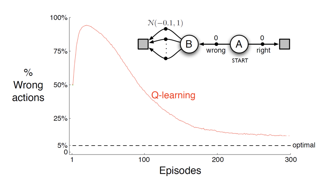
|
||||
|
||||
False signals from $\mathcal{N}(0.1,1)$, may have few positive results from random noise. (However, in the long run, it will converge to the expected negative value.)
|
||||
|
||||
#### Double Q-learning
|
||||
|
||||
(Hado van Hasselt 2010)
|
||||
|
||||
Train 2 action-value functions, Q1 and Q2
|
||||
|
||||
Do Q-learning on both, but
|
||||
|
||||
- never on the same time steps (Q1 and Q2 are indep.)
|
||||
- pick Q1 or Q2 at random to be updated on each step
|
||||
|
||||
If updating Q1, use Q2 for the value of the next state:
|
||||
|
||||
$$
|
||||
Q_1(S_t,A_t) \gets Q_1(S_t,A_t) + \alpha (R_{t+1} + \gamma Q_2(S_{t+1}, \arg\max_{a'\in A} Q_1(S_{t+1},a')) - Q_1(S_t,A_t))
|
||||
$$
|
||||
|
||||
Action selections are (say) $\epsilon$-greedy with respect to the sum of Q1 and Q2. (unbiased estimation and same convergence as Q-learning)
|
||||
|
||||
Drawbacks:
|
||||
|
||||
- More computationally expensive (only one function is trained at a time)
|
||||
|
||||
```pseudocode
|
||||
Initialize Q1 and Q2
|
||||
For each episode:
|
||||
Initialize state
|
||||
For each step:
|
||||
Choose $A$ from $S$ using policy derived from Q1 and Q2
|
||||
Take action $A$, observe $R$ and $S'$
|
||||
With probability $0.5$, update Q1:
|
||||
$Q1(S,A) \gets Q1(S,A) + \alpha (R + \gamma Q2(S', \arg\max_{a'\in A} Q1(S',a')) - Q1(S,A))$
|
||||
Otherwise, update Q2:
|
||||
$Q2(S,A) \gets Q2(S,A) + \alpha (R + \gamma Q1(S', \arg\max_{a'\in A} Q2(S',a')) - Q2(S,A))$
|
||||
$S \gets S'$
|
||||
End for
|
||||
End for
|
||||
```
|
||||
|
||||
#### Double DQN
|
||||
|
||||
(van Hasselt, Guez, Silver, 2015)
|
||||
|
||||
A better implementation of Double Q-learning.
|
||||
|
||||
- Dealing with maximization bias of Q-Learning
|
||||
- Current Q-network $w$ is used to select actions
|
||||
- Older Q-network $w^-$ is used to evaluate actions
|
||||
|
||||
$$
|
||||
l=\left(r+\gamma Q(s', \arg\max_{a'\in A} Q(s',a';w);w^-) - Q(s,a;w)\right)^2
|
||||
$$
|
||||
|
||||
Here $\arg\max_{a'\in A} Q(s',a';w)$ is the action selected by the current Q-network $w$.
|
||||
|
||||
$Q(s', \arg\max_{a'\in A} Q(s',a';w);w^-)$ is the action evaluation by the older Q-network $w^-$.
|
||||
|
||||
### Prioritized Experience Replay
|
||||
|
||||
(Schaul, Quan, Antonoglou, Silver, ICLR 2016)
|
||||
|
||||
Weight experience according to "surprise" (or error)
|
||||
|
||||
- Store experience in priority queue according to DQN error
|
||||
$$
|
||||
\left|r+\gamma \arg\max_{a'\in A} Q(s',a',w^-)-Q(s,a,w)\right|
|
||||
$$
|
||||
|
||||
- Stochastic Prioritization
|
||||
$$
|
||||
P(i)=\frac{p_i^\alpha}{\sum_k p_k^\alpha}
|
||||
$$
|
||||
- $p_i$ is proportional to the DQN error
|
||||
|
||||
- $\alpha$ determines how much prioritization is used, with $\alpha = 0$ corresponding to the uniform case.
|
||||
|
||||
### Dueling Q networks
|
||||
|
||||
(Wang et.al., ICML, 2016)
|
||||
|
||||
- Split Q-network into two channels
|
||||
|
||||
- Action-independent value function $V(s; w)$: measures how good is the state $s$
|
||||
|
||||
- Action-dependent advantage function $A(s, a; w)$: measure how much better is action $a$ than the average action in state $s$
|
||||
$$
|
||||
Q(s,a; w) = V(s; w) + A(s, a; w)
|
||||
$$
|
||||
|
||||
- Advantage function is defined as:
|
||||
$$
|
||||
A^\pi(s, a) = Q^\pi(s, a) - V^\pi(s)
|
||||
$$
|
||||
|
||||
The value stream learns to pay attention to the road
|
||||
|
||||
**The advantage stream**: pay attention only when there are cars immediately in front, so as to avoid collisions
|
||||
|
||||
### Multistep returns
|
||||
|
||||
Truncated n-step return from a state $s_t$
|
||||
|
||||
$$
|
||||
R^{n}_t = \sum_{i=0}^{n-1} \gamma^{(k)}_t R_{t+k+1}
|
||||
$$
|
||||
|
||||
Multistep Q-learning update rule:
|
||||
|
||||
$$
|
||||
I=\left(R^{n}_t + \gamma^{(n)}_t \max_{a'\in A} Q(s_{t+n},a';w)-Q(s,a,w)\right)^2
|
||||
$$
|
||||
|
||||
Singlestep Q-learning update rule:
|
||||
|
||||
$$
|
||||
I=\left(r+\gamma \max_{a'\in A} Q(s',a';w)-Q(s,a,w)\right)^2
|
||||
$$
|
||||
|
||||
### Distributed DQN
|
||||
|
||||
- Separating Learning from Acting
|
||||
- Distributing hundreds of actors over CPUs
|
||||
- Advantages: better harnessing computation, local priority evaluation, better exploration
|
||||
|
||||
#### Distributed DQN with Recurrent Experience Replay (R2D2)
|
||||
|
||||
Providing an LSTM layer after the convolutional stack
|
||||
|
||||
- To deal with partial observability
|
||||
|
||||
Other tricks:
|
||||
|
||||
- prioritized distributed replay
|
||||
- n-step double Q-learning (with n = 5)
|
||||
- generating experience by a large number of actors (typically 256)
|
||||
- learning from batches of replayed experience by a single learner
|
||||
|
||||
#### Agent 57
|
||||
|
||||
[link to paper](https://deepmind.google/discover/blog/agent57-outperforming-the-human-atari-benchmark/)
|
||||
@@ -1,300 +0,0 @@
|
||||
# CSE510 Deep Reinforcement Learning (Lecture 11)
|
||||
|
||||
> Materials Used
|
||||
>
|
||||
> - Much of the material and slides for this lecture were taken from Chapter 13 of Barto & Sutton textbook.
|
||||
>
|
||||
> - Some slides are borrowed from Rich Sutton’s RL class and David Silver's Deep RL tutorial
|
||||
|
||||
Problem: often the feature-based policies that work well (win games,
|
||||
maximize utilities) aren't the ones that approximate V / Q best
|
||||
|
||||
- Q-learning's priority: get Q-values close (modeling)
|
||||
- Action selection priority: get ordering of Q-values right (prediction)
|
||||
|
||||
Value functions can often be much more complex to represent than the
|
||||
corresponding policy
|
||||
|
||||
- Do we really care about knowing $Q(s, \text{left}) = 0.3554, Q(s, \text{right}) = 0.533$ Or just that "right is better than left in state $s$"
|
||||
|
||||
Motivates searching directly in a parameterized policy space
|
||||
|
||||
- Bypass learning value function and "directly" optimize the value of a policy
|
||||
|
||||
<details>
|
||||
<summary>Examples</summary>
|
||||
|
||||
Rock-Paper-Scissors
|
||||
|
||||
- Two-player game of rock-paper-scissors
|
||||
- Scissors beats paper
|
||||
- Rock beats scissors
|
||||
- Paper beats rock
|
||||
- Consider policies for iterated rock-paper-scissors
|
||||
- A deterministic policy is easily exploited
|
||||
- A uniform random policy is optimal (i.e., Nash equilibrium)
|
||||
|
||||
---
|
||||
|
||||
Partial Observable GridWorld
|
||||
|
||||

|
||||
|
||||
The agent cannot differentiate the grey state
|
||||
|
||||
Consider features of the following form (for all $N,E,S,W$ actions):
|
||||
|
||||
$$
|
||||
\phi(s,a)=1(\text{wall to} N, a=\text{move} E)
|
||||
$$
|
||||
|
||||
Compare value-based RL, suing an approximate value function
|
||||
|
||||
$$
|
||||
Q_\theta(s,a) = f(\phi(s,a),\theta)
|
||||
$$
|
||||
|
||||
To policy-based RL, using a parameterized policy
|
||||
|
||||
$$
|
||||
\pi_\theta(s,a) = g(\phi(s,a),\theta)
|
||||
$$
|
||||
|
||||
Under aliasing, an optimal deterministic policy will either
|
||||
|
||||
- move $W$ in both grey states (shown by red arrows)
|
||||
- move $E$ in both grey states
|
||||
|
||||
Either way, it can get stuck and _never_ reach the money
|
||||
|
||||
- Value-based RL learns a near-deterministic policy
|
||||
- e.g. greedy or $\epsilon$-greedy
|
||||
|
||||
So it will traverse the corridor for a long time
|
||||
|
||||
An optimal **stochastic** policy will randomly move $E$ or $W$ in grey cells.
|
||||
|
||||
$$
|
||||
\pi_\theta(\text{wall to }N\text{ and }S, \text{move }E) = 0.5\\
|
||||
\pi_\theta(\text{wall to }N\text{ and }S, \text{move }W) = 0.5
|
||||
$$
|
||||
|
||||
It will reach the goal state in a few steps with high probability
|
||||
|
||||
Policy-based RL can learn the optimal stochastic policy
|
||||
|
||||
</details>
|
||||
|
||||
## RL via Policy Gradient Ascent
|
||||
|
||||
The policy gradient approach has the following schema:
|
||||
|
||||
1. Select a space of parameterized policies (i.e., function class)
|
||||
2. Compute the gradient of the value of current policy wrt parameters
|
||||
3. Move parameters in the direction of the gradient
|
||||
4. Repeat these steps until we reach a local maxima
|
||||
|
||||
So we must answer the following questions:
|
||||
|
||||
- How should we represent and evaluate parameterized policies?
|
||||
- How can we compute the gradient?
|
||||
|
||||
### Policy learning objective
|
||||
|
||||
Goal: given policy $\pi_\theta(s,a)$ with parameter $\theta$, find best $\theta$
|
||||
|
||||
In episodic environments we can use the start value:
|
||||
|
||||
$$
|
||||
J_1(\theta) = V^{\pi_\theta}(s_1)=\mathbb{E}_{\pi_\theta}[v_1]
|
||||
$$
|
||||
|
||||
In continuing environments we can use the average value:
|
||||
|
||||
$$
|
||||
J_{avV}(\theta) = \sum_{s\in S} d^{\pi_\theta}(s) V^{\pi_\theta}(s)
|
||||
$$
|
||||
|
||||
Or the average reward per time-step
|
||||
|
||||
$$
|
||||
J_{avR}(\theta) = \sum_{s\in S} d^{\pi_\theta}(s) \sum_{a\in A} \pi_\theta(s,a) \mathcal{R}(s,a)
|
||||
$$
|
||||
|
||||
here $d^{\pi_\theta}(s)$ is the **stationary distribution** of Markov Chain for policy $\pi_\theta$.
|
||||
|
||||
### Policy optimization
|
||||
|
||||
Policy based reinforcement learning is an **optimization** problem
|
||||
|
||||
Find $\theta$ that maximises $J(\theta)$
|
||||
|
||||
Some approaches do not use gradient
|
||||
|
||||
- Hill climbing
|
||||
- Simplex / amoeba / Nelder Mead
|
||||
- Genetic algorithms
|
||||
|
||||
Greater efficiency often possible using gradient
|
||||
|
||||
- Gradient descent
|
||||
- Conjugate gradient
|
||||
- Quasi-newton
|
||||
|
||||
We focus on gradient descent, many extensions possible
|
||||
|
||||
And on methods that exploit sequential structure
|
||||
|
||||
### Policy gradient
|
||||
|
||||
Let $J(\theta)$ be any policy objective function
|
||||
|
||||
Policy gradient algorithms search for a _local_ maxima in $J(\theta)$ by ascending the gradient of the policy with respect to $\theta$
|
||||
|
||||
$$
|
||||
\Delta \theta = \alpha \nabla_\theta J(\theta)
|
||||
$$
|
||||
|
||||
Where $\nabla_\theta J(\theta)$ is the policy gradient.
|
||||
|
||||
$$
|
||||
\nabla_\theta J(\theta) = \begin{pmatrix}
|
||||
\frac{\partial J(\theta)}{\partial \theta_1} \\
|
||||
\frac{\partial J(\theta)}{\partial \theta_2} \\
|
||||
\vdots \\
|
||||
\frac{\partial J(\theta)}{\partial \theta_n}
|
||||
\end{pmatrix}
|
||||
$$
|
||||
|
||||
and $\alpha$ is the step-size parameter.
|
||||
|
||||
### Policy gradient methods
|
||||
|
||||
The main method we will introduce is Monte-Carlo policy gradient in Reinforcement Learning.
|
||||
|
||||
#### Score Function
|
||||
|
||||
Assume the policy $\pi_\theta$ is differentiable and non-zero and we know the gradient $\nabla_\theta \pi_\theta(s,a)$ for all $s\in S$ and $a\in A$.
|
||||
|
||||
We can compute the policy gradient analytically
|
||||
|
||||
We define the **Likelihood ratio** as:
|
||||
|
||||
$$
|
||||
\begin{aligned}
|
||||
\nabla_\theta \pi_\theta(s,a) = \pi_\theta(s,a) \frac{\nabla_\theta \pi_\theta(s,a)}{\pi_\theta(s,a)} \\
|
||||
&= \nabla_\theta \log \pi_\theta(s,a)
|
||||
\end{aligned}
|
||||
$$
|
||||
|
||||
The **Score Function** is:
|
||||
|
||||
$$
|
||||
\nabla_\theta \log \pi_\theta(s,a)
|
||||
$$
|
||||
|
||||
<details>
|
||||
<summary>Example</summary>
|
||||
|
||||
Take the softmax policy as example:
|
||||
|
||||
Weight actions using the linear combination of features $\phi(s,a)^\top\theta$:
|
||||
|
||||
Probability of action is proportional to the exponentiated weights:
|
||||
|
||||
$$
|
||||
\pi_\theta(s,a) \propto \exp(\phi(s,a)^\top\theta)
|
||||
$$
|
||||
|
||||
The score function is
|
||||
|
||||
$$
|
||||
\begin{aligned}
|
||||
\nabla_\theta \ln\left[\frac{\exp(\phi(s,a)^\top\theta)}{\sum_{a'\in A}\exp(\phi(s,a')^\top\theta)}\right] &= \nabla_\theta(\ln \exp(\phi(s,a)^\top\theta) - (\ln \sum_{a'\in A}\exp(\phi(s,a')^\top\theta))) \\
|
||||
&= \nabla_\theta\left(\phi(s,a)^\top\theta -\frac{\phi(s,a)\sum_{a'\in A}\exp(\phi(s,a')^\top\theta)}{\sum_{a'\in A}\exp(\phi(s,a')^\top\theta)}\right) \\
|
||||
&=\phi(s,a) - \sum_{a'\in A} \prod_\theta(s,a') \phi(s,a')
|
||||
&= \phi(s,a) - \mathbb{E}_{a'\sim \pi_\theta(s,a')}[\phi(s,a')]
|
||||
\end{aligned}
|
||||
$$
|
||||
|
||||
---
|
||||
|
||||
In continuous action spaces, a Gaussian policy is natural
|
||||
|
||||
Mean is a linear combination of state features $\mu(s) = \phi(s)^\top\theta$
|
||||
|
||||
Variance may be fixed $\sigma^2$, or can also parametrized
|
||||
|
||||
Policy is Gaussian, $a \sim N (\mu(s), \sigma^2)$
|
||||
|
||||
The score function is
|
||||
|
||||
$$
|
||||
\nabla_\theta \log \pi_\theta(s,a) = \frac{(a - \mu(s)) \phi(s)}{\sigma^2}
|
||||
$$
|
||||
|
||||
</details>
|
||||
|
||||
#### Policy Gradient Theorem
|
||||
|
||||
For any _differentiable_ policy $\pi_\theta(s,a)$,
|
||||
|
||||
for any of the policy objective function $J=J_1, J_{avR},$ or $\frac{1}{1-\gamma}J_{avV}$, the policy gradient is:
|
||||
|
||||
$$
|
||||
\nabla_\theta J(\theta) = \mathbb{\pi_\theta}[\nabla_\theta \log \pi_\theta(s,a) Q^{\pi_\theta}(s,a)]
|
||||
$$
|
||||
|
||||
<details>
|
||||
<summary>Proof</summary>
|
||||
|
||||
Take $\phi(s)=\sum_{a\in A} \nabla_\theta \pi_\theta(a|s)Q^{\pi}(s,a)$ to simplify the proof.
|
||||
|
||||
$$
|
||||
\begin{aligned}
|
||||
\nabla_\theta V^{\pi}(s)&=\nabla_\theta \left(\sum_{a\in A} \pi_\theta(a|s)Q^{\pi}(s,a)\right) \\
|
||||
&=\sum_{a\in A} \left(\nabla_\theta \pi_\theta(a|s)Q^{\pi}(s,a) + \pi_\theta(a|s) \nabla_\theta Q^{\pi}(s,a)\right) \text{by linear approximation}\\
|
||||
&=\sum_{a\in A} \left(\nabla_\theta \pi_\theta(a|s)Q^{\pi}(s,a) + \pi_\theta(a|s) \nabla_\theta \sum_{s',r\in S\times R} P(s',r|s,a) \left(r+V^{\pi}(s')\right)\right)\text{rewrite the Q-function as sum of expected rewards from actions} \\
|
||||
&=\sum_{a\in A} \left(\nabla_\theta \pi_\theta(a|s)Q^{\pi}(s,a) + \pi_\theta(a|s) \sum_{s',r\in S\times R} P(s',r|s,a) \nabla_\theta \left(r+V^{\pi}(s')\right)\right) \\
|
||||
&=\phi(s)+\sum_{a\in A} \left(\pi_\theta(a|s) \sum_{s'\in S} P(s'|s,a) \nabla_\theta V^{\pi}(s')\right) \\
|
||||
&=\phi(s)+\sum_{s\in S} \sum_{a\in A} \pi_\theta(a|s) P(s'|s,a) \nabla_\theta V^{\pi}(s') \\
|
||||
&=\phi(s)+\sum_{s\in S} \rho(s\to s',1)\nabla_\theta V^{\pi}(s') \text{ notice the recurrence relation}\\
|
||||
&=\phi(s)+\sum_{s'\in S} \rho(s\to s',1)\left[\phi(s')+\sum_{s''\in S} \rho(s'\to s'',1)\nabla_\theta V^{\pi}(s'')\right] \\
|
||||
&=\phi(s)+\left[\sum_{s'\in S} \rho(s\to s',1)\phi(s')\right]+\left[\sum_{s''\in S} \rho(s\to s'',2)\nabla_\theta V^{\pi}(s'')\right] \\
|
||||
&=\cdots\\
|
||||
&=\sum_{x\in S}\sum_{k=0}^\infty \rho(s\to x,k)\phi(x)
|
||||
\end{aligned}
|
||||
$$
|
||||
|
||||
Just to note that $\rho(s\to x,k)=\sum_{a\in A} \pi_\theta(a|s) P(x|s,a)^k$ is the probability of reaching state $x$ in $k$ steps from state $s$.
|
||||
|
||||
Let $\eta(s)=\sum_{k=0}^\infty \rho(s_0\to s,k)$ be the expected number of steps to reach state $s$ from state $s_0$.
|
||||
|
||||
Note that $\sum_{s\in S} \eta(s)$ is constant depends solely on the initial state $s_0$ and policy $\pi_\theta$.
|
||||
|
||||
So $d^{\pi_\theta}(s)=\frac{\eta(s)}{\sum_{s'\in S} \eta(s')}$ is the stationary distribution of the Markov Chain for policy $\pi_\theta$.
|
||||
|
||||
$$
|
||||
\begin{aligned}
|
||||
\nabla_\theta J(\theta)&=\nabla_\theta V^{\pi}(s_0)\\
|
||||
&=\sum_{s\in S} \sum_{k=0}^\infty \rho(s_0\to s,k)\phi(s)\\
|
||||
&=\sum_{s\in S} \eta(s)\phi(s)\\
|
||||
&=\sum_{s\in S} \eta(s)\sum_{a\in A} \frac{\eta(s)}{\sum_{s'\in S} \eta(s')}\phi(s)\\
|
||||
&\propto \sum_{s\in S} \frac{\eta(s)}{\sum_{s'\in S} \eta(s')}\phi(s)\\
|
||||
&=\sum_{s\in S} d^{\pi_\theta}(s)\sum_{a\in A} \nabla_\theta \pi_\theta(a|s)Q^{\pi_\theta}(s,a)\\
|
||||
&=\left[\sum_{s\in S} d^{\pi_\theta}(s)\sum_{a\in A} \pi_\theta(a|s)\right]\nabla_\theta Q^{\pi_\theta}(s,a)\\
|
||||
&= \mathbb{E}_{\pi_\theta}[\nabla_\theta \log \pi_\theta(s,a) Q^{\pi_\theta}(s,a)]
|
||||
\end{aligned}
|
||||
$$
|
||||
|
||||
</details>
|
||||
|
||||
#### Monte-Carlo Policy Gradient
|
||||
|
||||
We can use the score function to compute the policy gradient.
|
||||
|
||||
## Actor-Critic methods
|
||||
|
||||
### Q Actor-Critic
|
||||
|
||||
### Advantage Actor-Critic
|
||||
@@ -1,204 +0,0 @@
|
||||
# CSE510 Deep Reinforcement Learning (Lecture 12)
|
||||
|
||||
## Policy Gradient Theorem
|
||||
|
||||
For any differentiable policy $\pi_\theta(s,a)$, for any o the policy objective functions $J=J_1, J_{avR}$ or $\frac{1}{1-\gamma} J_{avV}$
|
||||
|
||||
The policy gradient is
|
||||
|
||||
$$
|
||||
\nabla_{\theta}J(\theta)=\mathbb{E}_{\pi_{\theta}}\left[\nabla_\theta \log \pi_\theta(s,a)Q^{\pi_\theta}(s,a)\right]
|
||||
$$
|
||||
|
||||
## Policy Gradient Methods
|
||||
|
||||
Advantages of Policy-Based RL
|
||||
|
||||
Advantages:
|
||||
|
||||
- Better convergence properties
|
||||
- Effective in high-dimensional or continuous action spaces
|
||||
- Can learn stochastic policies
|
||||
|
||||
Disadvantages:
|
||||
|
||||
- Typically converge to a local rather than global optimum
|
||||
- Evaluating a policy is typically inefficient and high variance
|
||||
|
||||
### Anchor-Critic Methods
|
||||
|
||||
#### Q Actor-Critic
|
||||
|
||||
Reducing Variance Using a Critic
|
||||
|
||||
Monte-Carlo Policy Gradient still has high variance.
|
||||
|
||||
We use a critic to estimate the action-value function $Q_w(s,a)\approx Q^{\pi_\theta}(s,a)$.
|
||||
|
||||
Anchor-critic algorithms maintain two sets of parameters:
|
||||
|
||||
Critic: updates action-value function parameters $w$
|
||||
|
||||
Actor: updates policy parameters $\theta$, in direction suggested by the critic.
|
||||
|
||||
Actor-critic algorithms follow an approximate policy gradient:
|
||||
|
||||
$$
|
||||
\nabla_\theta J(\theta) \approx \mathbb{E}_{\pi_{\theta}}\left[\nabla_\theta \log \pi_\theta(s,a)Q_w(s,a)\right]
|
||||
$$
|
||||
$$
|
||||
\Delta \theta = \alpha \nabla_\theta \log \pi_\theta(s,a)Q_w(s,a)
|
||||
$$
|
||||
|
||||
Action-Value Actor-Critic
|
||||
|
||||
- Simple actor-critic algorithm based on action-value critic
|
||||
- Using linear value function approximation $Q_w(s,a)=\phi(s,a)^\top w$
|
||||
|
||||
Critic: updates $w$ by linear $TD(0)$
|
||||
Actor: updates $\theta$ by policy gradient
|
||||
|
||||
```python
|
||||
def Q_actor-critic(states,theta):
|
||||
actions=sample_actions(a,pi_theta)
|
||||
for i in range(num_steps):
|
||||
reward=sample_rewards(actions,states)
|
||||
transition=sample_transition(actions,states)
|
||||
new_actions=sample_action(transition,theta)
|
||||
delta=sample_reward+gamma*Q_w(transition, new_actions)-Q_w(states, actions)
|
||||
theta=theta+alpha*nabla_theta*log(pi_theta(states, actions))*Q_w(states, actions)
|
||||
w=w+beta*delta*phi(states, actions)
|
||||
a=new_actions
|
||||
s=transition
|
||||
```
|
||||
|
||||
#### Advantage Actor-Critic
|
||||
|
||||
Reducing variance using a baseline
|
||||
|
||||
- We subtract a baseline function $B(s)$ form the policy gradient
|
||||
- This can reduce the variance without changing expectation
|
||||
|
||||
$$
|
||||
\begin{aligned}
|
||||
\mathbb{E}_{\pi_\theta}\left[\nabla_\theta\log \pi_\theta(s,a)B(s)\right]&=\sum_{s\in S}d^{\pi_\theta}(s)\sum_{a\in A}\nabla_{\theta}\pi_\theta(s,a)B(s)\\
|
||||
&=\sum_{s\in S}d^{\pi_\theta}B(s)\nabla_\theta\sum_{a\in A}\pi_\theta(s,a)\\
|
||||
&=0
|
||||
\end{aligned}
|
||||
$$
|
||||
|
||||
A good baseline is the state value function $B(s)=V^{\pi_\theta}(s)$
|
||||
|
||||
So we can rewrite the policy gradient using the advantage function $A^{\pi_\theta}(s,a)=Q^{\pi_\theta}(s,a)-V^{\pi_theta}(s)$
|
||||
|
||||
$$
|
||||
\nabla_\theta J(\theta)=\mathbb{E}\left[\nabla_\theta \log \pi_\theta(s,a) A^{\pi_theta}(s,a)\right]
|
||||
$$
|
||||
|
||||
##### Estimating the Advantage function
|
||||
|
||||
**Method 1:** direct estimation
|
||||
|
||||
> May increase the variance
|
||||
|
||||
The advantage function can significantly reduce variance of policy gradient
|
||||
|
||||
So the critic should really estimate the advantage function
|
||||
|
||||
For example, by estimating both $V^{\pi_theta}(s)$ and $Q^{\pi_theta}(s,a)$
|
||||
|
||||
Using two function approximators and two parameter vectors,
|
||||
|
||||
$$
|
||||
V_v(s)\approx V^{\pi_\theta}(s)\\
|
||||
Q_w(s,a)\approx Q^{\pi_\theta}(s,a)\\
|
||||
A(s,a)=Q_w(s,a)-V_v(s)
|
||||
$$
|
||||
|
||||
And updating both value functions by e.g. TD learning
|
||||
|
||||
**Method 2:** using the TD error
|
||||
|
||||
> We can prove that TD error is an unbiased estimation of the advantage function
|
||||
|
||||
For the true value function $V^{\pi_\theta}(s)$, the TD error $\delta^{\pi_\theta}$
|
||||
|
||||
$$
|
||||
\delta^{\pi_\theta} = r + \gamma V^{\pi_\theta}(s) - V^{\pi_\theta}(s)
|
||||
$$
|
||||
|
||||
is an unbiased estimate of the advantage function
|
||||
|
||||
$$
|
||||
\begin{aligned}
|
||||
\mathbb{E}_{\pi_\theta}[\delta^{\pi_\theta}| s,a]&=\mathbb{E}_{\pi_\theta}[r + \gamma V^{\pi_\theta}(s') |s,a]-V^{\pi_\theta}(s)\\
|
||||
&=Q^{\pi_\theta}(s,a)-V^{\pi_\theta}(s)\\
|
||||
&=A^{\pi_\theta}(s,a)
|
||||
\end{aligned}
|
||||
$$
|
||||
|
||||
So we can use the TD error to compute the policy gradient
|
||||
|
||||
$$
|
||||
\Delta \theta J(\theta) = \mathbb{E}_{\pi_\theta}[\nabla_\theta \log \pi_\theta(s,a) \delta^{\pi_\theta}]
|
||||
$$
|
||||
|
||||
In practice, we can use an approximate TD error $\delta_v=r+\gamma V_v(s')-V_v(s)$ to compute the policy gradient
|
||||
|
||||
### Summary of policy gradient algorithms
|
||||
|
||||
THe policy gradient has many equivalent forms.
|
||||
|
||||
$$
|
||||
\begin{aligned}
|
||||
\nabla_\theta J(\theta) &= \mathbb{E}_{\pi_\theta}[\nabla_\theta \log \pi_\theta(s,a) v_t] \text{ REINFORCE} \\
|
||||
&= \mathbb{E}_{\pi_\theta}[\nabla_\theta \log \pi_\theta(s,a) Q_w(s,a)] \text{ Q Actor-Critic} \\
|
||||
&= \mathbb{E}_{\pi_\theta}[\nabla_\theta \log \pi_\theta(s,a) A^{\pi_\theta}(s,a)] \text{ Advantage Actor-Critic} \\
|
||||
&= \mathbb{E}_{\pi_\theta}[\nabla_\theta \log \pi_\theta(s,a) \delta^{\pi_\theta}] \text{ TD Actor-Critic}
|
||||
\end{aligned}
|
||||
$$
|
||||
|
||||
Each leads s stochastic gradient ascent algorithm.
|
||||
|
||||
Critic use policy evaluation to estimate the $Q^\pi(s,a)$ or $A^\pi(s,a)$ or $V^\pi(s)$.
|
||||
|
||||
## Compatible Function Approximation
|
||||
|
||||
If the following two conditions are satisfied:
|
||||
|
||||
1. Value function approximation is a compatible with the policy
|
||||
$$
|
||||
\nabla_w Q_w(s,a) = \nabla_\theta \log \pi_\theta(s,a)
|
||||
$$
|
||||
2. Value function parameters $w$ minimize the MSE
|
||||
$$
|
||||
\epsilon = \mathbb{E}_{\pi_\theta}[(Q^{\pi_\theta}(s,a)-Q_w(s,a))^2]
|
||||
$$
|
||||
Note $\epsilon$ need not be zero, just need to be minimized.
|
||||
|
||||
Then the policy gradient is exact
|
||||
|
||||
$$
|
||||
\nabla_\theta J(\theta) = \mathbb{E}_{\pi_\theta}[\nabla_\theta \log \pi_\theta(s,a) Q_w(s,a)]
|
||||
$$
|
||||
|
||||
Remember:
|
||||
|
||||
$$
|
||||
\nabla_\theta J(\theta) = \mathbb{E}_{\pi_\theta}[\nabla_\theta \log \pi_\theta(s,a) Q^{\pi_\theta}(s,a)]
|
||||
$$
|
||||
|
||||
### Challenges with Policy Gradient Methods
|
||||
|
||||
- Data Inefficiency
|
||||
- On-policy method: for each new policy, we need to generate a completely new
|
||||
- trajectory
|
||||
- The data is thrown out after just one gradient update
|
||||
- As complex neural networks need many updates, this makes the training process very slow
|
||||
- Unstable update: step size is very important
|
||||
- If step size is too large:
|
||||
- Large step -> bad policy
|
||||
- Next batch is generated from current bad policy -> collect bad samples
|
||||
- Bad samples -> worse policy (compare to supervised learning: the correct label and data in the following batches may correct it)
|
||||
- If step size is too small: the learning process is slow
|
||||
|
||||
@@ -1,229 +0,0 @@
|
||||
# CSE510 Deep Reinforcement Learning (Lecture 13)
|
||||
|
||||
> Recap from last lecture
|
||||
>
|
||||
> For any differentiable policy $\pi_\theta(s,a)$, for any o the policy objective functions $J=J_1, J_{avR}$ or $\frac{1}{1-\gamma} J_{avV}$
|
||||
>
|
||||
> The policy gradient is
|
||||
>
|
||||
> $\nabla_{\theta}J(\theta)=\mathbb{E}_{\pi_{\theta}}\left[\nabla_\theta \log \pi_\theta(s,a)Q^{\pi_\theta}(s,a)\right]$
|
||||
|
||||
## Problem for policy gradient method
|
||||
|
||||
Data Inefficiency
|
||||
|
||||
- On-policy method: for each new policy, we need to generate a completely new trajectory
|
||||
- The data is thrown out after just one gradient update
|
||||
- As complex neural networks need many updates, this makes the training process very slow
|
||||
|
||||
Unstable update: step size is very important
|
||||
|
||||
- If step size is too large:
|
||||
- Large step -> bad policy
|
||||
- Next batch is generated from current bad policy → collect bad samples
|
||||
- Bad samples -> worse policy (compare to supervised learning: the correct label and data in the following batches may correct it)
|
||||
- If step size is too small: the learning process is slow
|
||||
|
||||
## Deriving the optimization objection function of Trusted Region Policy Optimization (TRPO)
|
||||
|
||||
### Objective of Policy Gradient Methods
|
||||
|
||||
Policy Objective
|
||||
|
||||
$$
|
||||
J(\pi_\theta)=\mathbb{E}_{\tau\sim \pi_theta}\sum_{t=0}^{\infty} \gamma^t r^t
|
||||
$$
|
||||
|
||||
here $\tau$ is the trajectory for the policy $\pi_\theta$.
|
||||
|
||||
Policy objective can be written in terms of old one:
|
||||
|
||||
$$
|
||||
J(\pi_{\theta'})-J(\pi_{\theta})=\mathbb{E}_{\tau \sim \pi_{\theta'}}\sum_{t=0}^{\infty}\gamma^t A^{\pi_\theta}(s_t,a_t)
|
||||
$$
|
||||
|
||||
Equivalently for succinctness:
|
||||
|
||||
$$
|
||||
J(\pi')-J(\pi)=\mathbb{E}_{\tau\in \pi'}\sum_{t=0}^{\infty} A^{\pi}(s_t,a_t)
|
||||
$$
|
||||
|
||||
<details>
|
||||
<summary> Proof</summary>
|
||||
|
||||
$$
|
||||
\begin{aligned}
|
||||
&\mathbb{E}_{\tau\sim \pi'}\left[\gamma^t A^{\pi_\theta}(s_t,a_t)\right]\\
|
||||
&=E_{\tau\sim \pi'}\left[\sum_{t=0}^{\infty}\gamma^t R(s_0)+\sum_{t=0}^{\infty} \gamma^{t+1}V^{\pi}(s_{t+1})-\sum_{t=0}^{\infty} \gamma^{t}V^\pi(s_t)\right]\\
|
||||
&=J(\pi')+\sum_{t=1}^{\infty} \gamma^{t}V^{\pi}(s_t)-\sum_{t=0}^{\infty} \gamma^{t}V^\pi(s_t)\\
|
||||
&=J(\pi')-\mathbb{E}_{\tau\sim\pi'}V^{\pi}(s_0)\\
|
||||
&=J(\pi')-J(\pi)
|
||||
\end{aligned}
|
||||
$$
|
||||
|
||||
</details>
|
||||
|
||||
### Importance Sampling
|
||||
|
||||
Estimate one distribution by sampling form anther distribution
|
||||
|
||||
$$
|
||||
\begin{aligned}
|
||||
\mathbb{E}_{x\sim p}[f(x)]&=\int f(x)p(x)dx
|
||||
&=\int f(x)\frac{p(x)}{q(x)}q(x)dx\\
|
||||
&=\mathbb{E}_{x\sim q}\left[f(x)\frac{p(x)}{q(x)}\right]\\
|
||||
&\approx \frac{1}{N}\sum_{i=1,x^i\in q}^N f(x^i)\frac{p(x^i)}{q(x^i)}
|
||||
\end{aligned}
|
||||
$$
|
||||
|
||||
### Estimating objective with importance sampling
|
||||
|
||||
Discounted state visit distribution:
|
||||
|
||||
$$
|
||||
d^\pi(s)=(1-\gamma)\sum_{t=0}^{\infty}\gamma^t P(s_t=s|\pi)
|
||||
$$
|
||||
|
||||
$$
|
||||
\begin{aligned}
|
||||
J(\pi')-J(\pi)&=\mathbb{E}_{\tau\sim\pi'}\sum_{t=0}^{\infty} \gamma^t A^{\pi}(s_t,a_t)\\
|
||||
&=\mathbb{E}_{s\sim d^{\pi'}, a\sim \pi'} A^{\pi}(s,a)\\
|
||||
&=\mathbb{E}_{s\sim d^{\pi'}, a\sim \pi}\left[A^{\pi'}(s,a)\frac{\pi'(a|s)}{\pi(a|s)}\right]\\
|
||||
\end{aligned}
|
||||
$$
|
||||
|
||||
Using the old policy to sample states form a policy that we are trying to optimize.
|
||||
|
||||
$$
|
||||
L_\pi(\pi')=\mathbb{E}_{s\sim d^{\pi'}, a\sim \pi}\left[A^{\pi'}(s,a)\frac{\pi'(a|s)}{\pi(a|s)}\right]
|
||||
$$
|
||||
|
||||
### Lower bound of Optimization
|
||||
|
||||
> [!NOTE]
|
||||
>
|
||||
> (Kullback-Leibler) KL divergence is a measure of the difference between two probability distributions.
|
||||
>
|
||||
> $D_{KL}(\pi(\dot|s)||\pi'(\dot|s))=\int_s \pi(a|s)\log \frac{\pi(a|s)}{\pi'(a|s)}da$
|
||||
|
||||
$$
|
||||
J(\pi')-J(\pi)\geq L_\pi(\pi')-C\max_{s\in S}D_{KL}(\pi(\dot|s)||\pi'(\dot|s))
|
||||
$$
|
||||
|
||||
where $C$ is a constant.
|
||||
|
||||
Optimizing the objective function:
|
||||
|
||||
$$
|
||||
\max_{\pi'} J(\pi')-J(\pi)
|
||||
$$
|
||||
|
||||
By maximizing the lower bound
|
||||
|
||||
$$
|
||||
\max_{\pi'} L_\pi(\pi')-C\max_{s\in S}D_{KL}(\pi(\dot|s)||\pi'(\dot|s))
|
||||
$$
|
||||
|
||||
### Monotonic Improvement Theorem
|
||||
|
||||
Proof of improvement guarantee: Suppose $\pi_{k+1}$ and $\pi_k$ are related by
|
||||
|
||||
$$
|
||||
\pi_{k+1}=\max_{\pi'} L_\pi(\pi')-C\max_{s\in S}D_{KL}(\pi(\dot|s)||\pi'(\dot|s))
|
||||
$$
|
||||
|
||||
$\pi_{k}$ is a feasible point, and the objective at $\pi_k$ is equal to 0.
|
||||
|
||||
$$
|
||||
L_{\pi_k}(\pi_{k})\propto \mathbb{E}_{s,a\sim d^{\pi_k}}[A^{\pi_k}(s,a)]=0
|
||||
$$
|
||||
$$
|
||||
D_{KL}(\pi_k||\pi_k)[s]=0
|
||||
$$
|
||||
|
||||
Optimal value $\geq 0$.
|
||||
|
||||
By the performance bound, $J_{pi_{k+1}}-J_{pi_k}\geq 0$.
|
||||
|
||||
### Final objective function
|
||||
|
||||
$$
|
||||
\max_{\pi'}\mathbb{E}_{s\sim d^{\pi}, a\sim \pi}[A^{\pi'}(s,a)\frac{\pi'(a|s)}{\pi(a|s)}]-C\max_{s\in S}D_{KL}(\pi(\dot|s)||\pi'(\dot|s))
|
||||
$$
|
||||
|
||||
by approximation
|
||||
|
||||
$$
|
||||
\max_{\pi'}\mathbb{E}_{s\sim d^{\pi}, a\sim \pi}[A^{\pi'}(s,a)\frac{\pi'(a|s)}{\pi(a|s)}]-C\mathbb{E}_{s\in S}D_{KL}(\pi(\dot|s)||\pi'(\dot|s))
|
||||
$$
|
||||
|
||||
With the Lagrangian Duality, the objective is mathematically the same as following using a trust region constraint:
|
||||
|
||||
$$
|
||||
\max_{\pi'} L_\pi(\pi')
|
||||
$$
|
||||
|
||||
such that
|
||||
|
||||
$$
|
||||
\mathbb{E}_{s\in S}D_{KL}(\pi(\dot|s)||\pi'(\dot|s))\leq \delta
|
||||
$$
|
||||
|
||||
$C$ gets very high when $\gamma$ is close to one and the corresponding gradient step size becomes too small.
|
||||
|
||||
$$
|
||||
C\propto \frac{\epsilon \gamma}{(1-\gamma)^2}
|
||||
$$
|
||||
|
||||
- Empirical results show that it needs to more adaptive
|
||||
- But Tuning $C$ is hard (need some trick just like PPO)
|
||||
- TRPO uses trust region constraint and make $\delta$ a tunable hyperparameter.
|
||||
|
||||
## Trust Region Policy Optimization (TRPO)
|
||||
|
||||
$$
|
||||
\max_{\pi'} L_\pi(\pi')
|
||||
$$
|
||||
|
||||
such that
|
||||
|
||||
$$
|
||||
\mathbb{E}_{s\in S}D_{KL}(\pi(\dot|s)||\pi'(\dot|s))\leq \delta
|
||||
$$
|
||||
|
||||
Make linear approximation to $L_{\pi_{\theta_{old}}}$ and quadratic approximation to KL term.
|
||||
|
||||
Maximize $g\cdot(\theta-\theta_{old})-\frac{\beta}{2}(\theta-\theta_{old})^\top F(\theta-\theta_{old})$
|
||||
|
||||
where $g=\frac{\partial}{\partial \theta}L_{\pi_{\theta_{old}}}(\pi_{\theta})\vert_{\theta=\theta_{old}}$ and $F=\frac{\partial^2}{\partial \theta^2}\overline{KL}_{\pi_{\theta_{old}}}(\pi_{\theta})\vert_{\theta=\theta_{old}}$
|
||||
|
||||
<details>
|
||||
<summary>Taylor Expansion of KL Term</summary>
|
||||
|
||||
$$
|
||||
D_{KL}(\pi_{\theta_{old}}|\pi_{\theta})\approx D_{KL}(\pi_{\theta_{old}}|\pi_{\theta_{old}})+d^\top \nabla_\theta D_{KL}(\pi_{\theta_{old}}|\pi_{\theta})\vert_{\theta=\theta_{old}}+\frac{1}{2}d^\top \nabla_\theta^2 D_{KL}(\pi_{\theta_{old}}|\pi_{\theta})\vert_{\theta=\theta_{old}}d
|
||||
$$
|
||||
|
||||
$$
|
||||
\begin{aligned}
|
||||
\nabla_\theta D_{KL}(\pi_{\theta_{old}}|\pi_{\theta})&=-\nabla_\theta \mathbb{E}_{x\sim \pi_{\theta_{old}}}\log P_\theta(x)\vert_{\theta=\theta_{old}}\\
|
||||
&=-\mathbb{E}_{x\sim \pi_{\theta_{old}}}\nabla_\theta \log P_\theta(x)\vert_{\theta=\theta_{old}}\\
|
||||
&=-\mathbb{E}_{x\sim \pi_{\theta_{old}}}\frac{1}{\pi_{\theta_{old}}(x)}\nabla_\theta P_\theta(x)\vert_{\theta=\theta_{old}}\\
|
||||
&=\int_x P_{\theta_{old}}(x)\frac{1}{P_{\theta_{old}}(x)}\nabla_\theta P_\theta(x)\vert_{\theta=\theta_{old}} dx\\
|
||||
&=\int_x P_{\theta_{old}}(x)\nabla_\theta P_\theta(x)\vert_{\theta=\theta_{old}} dx\\
|
||||
&=\nabla_\theta \int_x P_{\theta_{old}}(x) \vert_{\theta=\theta_{old}} dx\\
|
||||
&=0
|
||||
\end{aligned}
|
||||
$$
|
||||
|
||||
$$
|
||||
\begin{aligned}
|
||||
\nabla_\theta^2 D_{KL}(\pi_{\theta_{old}}|\pi_{\theta})\vert_{\theta=\theta_{old}}&=-\mathbb{E}_{x\sim \pi_{\theta_{old}}}\nabla_\theta^2 \log P_\theta(x)\vert_{\theta=\theta_{old}}\\
|
||||
&=-\mathbb{E}_{x\sim \pi_{\theta_{old}}}\nabla_\theta \left(\frac{\nabla_\theta P_\theta(x)}{P_\theta(x)}\right)\vert_{\theta=\theta_{old}}\\
|
||||
&=-\mathbb{E}_{x\sim \pi_{\theta_{old}}}\left(\frac{\nabla_\theta^2 P_\theta(x)-\nabla_\theta P_\theta(x)\nabla_\theta P_\theta(x)^\top}{P_\theta(x)^2}\right)\vert_{\theta=\theta_{old}}\\
|
||||
&=-\mathbb{E}_{x\sim \pi_{\theta_{old}}}\left(\frac{\nabla_\theta^2 P_\theta(x)\vert_{\theta=\theta_{old}}}P_{\theta_{old}}(x)\right)+\mathbb{E}_{x\sim \pi_{\theta_{old}}}\left(\nabla_\theta \log P_\theta(x)\nabla_\theta \log P_\theta(x)^\top\right)\vert_{\theta=\theta_{old}}\\
|
||||
&=\mathbb{E}_{x\sim \pi_{\theta_{old}}}\nabla_\theta\log P_\theta(x)\nabla_\theta\log P_\theta(x)^\top\vert_{\theta=\theta_{old}}\\
|
||||
\end{aligned}
|
||||
$$
|
||||
|
||||
</details>
|
||||
@@ -1,182 +0,0 @@
|
||||
# CSE510 Deep Reinforcement Learning (Lecture 14)
|
||||
|
||||
## Advanced Policy Gradient Methods
|
||||
|
||||
### Trust Region Policy Optimization (TRPO)
|
||||
|
||||
"Recall" from last lecture
|
||||
|
||||
$$
|
||||
\max_{\pi'} \mathbb{E}_{s\sim d^{\pi},a\sim \pi} \left[\frac{\pi'(a|s)}{\pi(a|s)}A^{\pi}(s,a)\right]
|
||||
$$
|
||||
|
||||
such that
|
||||
|
||||
$$
|
||||
\mathbb{E}_{s\sim d^{\pi}} D_{KL}(\pi(\dot|s)||\pi'(\dot|s))\leq \delta
|
||||
$$
|
||||
|
||||
Unconstrained penalized objective:
|
||||
|
||||
$$
|
||||
d^*=\arg\max_{d} J(\theta+d)-\lambda(D_{KL}\left[\pi_\theta||\pi_{\theta+d}\right]-\delta)
|
||||
$$
|
||||
|
||||
$\theta_{new}=\theta_{old}+d$
|
||||
|
||||
First order Taylor expansion for the loss and second order for the KL:
|
||||
|
||||
$$
|
||||
\approx \arg\max_{d} J(\theta_{old})+\nabla_\theta J(\theta)\mid_{\theta=\theta_{old}}d-\frac{1}{2}\lambda(d^\top\nabla_\theta^2 D_{KL}\left[\pi_{\theta_{old}}||\pi_{\theta}\right]\mid_{\theta=\theta_{old}}d)+\lambda \delta
|
||||
$$
|
||||
|
||||
If you are really interested, try to fill the solving the KL Constrained Problem section.
|
||||
|
||||
#### Natural Gradient Descent
|
||||
|
||||
Setting the gradient to zero:
|
||||
|
||||
$$
|
||||
\begin{aligned}
|
||||
0&=\frac{\partial}{\partial d}\left(-\nabla_\theta J(\theta)\mid_{\theta=\theta_{old}}d+\frac{1}{2}\lambda(d^\top F(\theta_{old})d\right)\\
|
||||
&=-\nabla_\theta J(\theta)\mid_{\theta=\theta_{old}}+\frac{1}{2}\lambda F(\theta_{old})d
|
||||
\end{aligned}
|
||||
$$
|
||||
|
||||
$$
|
||||
d=\frac{2}{\lambda} F^{-1}(\theta_{old})\nabla_\theta J(\theta)\mid_{\theta=\theta_{old}}
|
||||
$$
|
||||
|
||||
The natural gradient is
|
||||
|
||||
$$
|
||||
\tilde{\nabla}J(\theta)=F^{-1}(\theta_{old})\nabla_\theta J(\theta)
|
||||
$$
|
||||
|
||||
$$
|
||||
\theta_{new}=\theta_{old}+\alpha F^{-1}(\theta_{old})\hat{g}
|
||||
$$
|
||||
|
||||
$$
|
||||
D_{KL}(\pi_{\theta_{old}}||\pi_{\theta})\approx \frac{1}{2}(\theta-\theta_{old})^\top F(\theta_{old})(\theta-\theta_{old})
|
||||
$$
|
||||
|
||||
$$
|
||||
\frac{1}{2}(\alpha g_N)^\top F(\alpha g_N)=\delta
|
||||
$$
|
||||
|
||||
$$
|
||||
\alpha=\sqrt{\frac{2\delta}{g_N^\top F g_N}}
|
||||
$$
|
||||
|
||||
However, due to the quadratic approximation, the KL constrains may be violated.
|
||||
|
||||
#### Linear search
|
||||
|
||||
We do Linear search for the best step size by making sure that
|
||||
|
||||
- Improving the objective
|
||||
- Satisfying the KL constraint
|
||||
|
||||
TRPO = NPG + Linesearch + monotonic improvement theorem
|
||||
|
||||
#### Summary of TRPO
|
||||
|
||||
Pros
|
||||
|
||||
- Proper learning step
|
||||
- [Monotonic improvement guarantee](./CSE510_L13.md#Monotonic-Improvement-Theorem)
|
||||
|
||||
Cons
|
||||
|
||||
- Poor scalability
|
||||
- Second-order optimization: computing Fisher Information Matrix and its inverse every time for the current policy model is expensive
|
||||
- Not quite sample efficient
|
||||
- Requiring a large batch of rollouts to approximate accurately
|
||||
|
||||
### Proximal Policy Optimization (PPO)
|
||||
|
||||
> Proximal Policy Optimization (PPO), which perform comparably or better than state-of-the-art approaches while being much simpler to implement and tune. -- OpenAI
|
||||
|
||||
[link to paper](https://arxiv.org/pdf/1707.06347)
|
||||
|
||||
Idea:
|
||||
|
||||
- The constraint helps in the training process. However, maybe the constraint is not a strict constraint:
|
||||
- Does it matter if we only break the constraint just a few times?
|
||||
|
||||
What if we treat it as a “soft” constraint? Add proximal value to the objective function?
|
||||
|
||||
#### PPO with Adaptive KL Penalty
|
||||
|
||||
$$
|
||||
\max_{\theta} \hat{\mathbb{E}_t}\left[\frac{\pi_\theta(a_t|s_t)}{\pi_{\theta_{old}}(a_t|s_t)}\hat{A}_t\right]-\beta \hat{\mathbb{E}_t}\left[KL[\pi_{\theta_{old}}(\dot|s_t),\pi_{\theta}(\dot|s_t)]\right]
|
||||
$$
|
||||
|
||||
Use adaptive $\beta$ value.
|
||||
|
||||
$$
|
||||
L^{KLPEN}(\theta)=\hat{\mathbb{E}_t}\left[\frac{\pi_\theta(a_t|s_t)}{\pi_{\theta_{old}}(a_t|s_t)}\hat{A}_t\right]-\beta \hat{\mathbb{E}_t}\left[KL[\pi_{\theta_{old}}(\dot|s_t),\pi_{\theta}(\dot|s_t)]\right]
|
||||
$$
|
||||
|
||||
Compute $d=\hat{\mathbb{E}_t}\left[KL[\pi_{\theta_{old}}(\dot|s_t),\pi_{\theta}(\dot|s_t)]\right]$
|
||||
|
||||
- If $d<d_{target}/1.5$, $\beta\gets \beta/2$
|
||||
- If $d>d_{target}\times 1.5$, $\beta\gets \beta\times 2$
|
||||
|
||||
#### PPO with Clipped Objective
|
||||
|
||||
$$
|
||||
\max_{\theta} \hat{\mathbb{E}_t}\left[\frac{\pi_\theta(a_t|s_t)}{\pi_{\theta_{old}}(a_t|s_t)}\hat{A}_t\right]
|
||||
$$
|
||||
|
||||
$$
|
||||
r_t(\theta)=\frac{\pi_\theta(a_t|s_t)}{\pi_{\theta_{old}}(a_t|s_t)}
|
||||
$$
|
||||
|
||||
- Here, $r_t(\theta)$ measures how much the new policy changes the probability of taking action $a_t$ in state $s_t$:
|
||||
- If $r_t > 1$ :the action becomes more likely under the new policy.
|
||||
- If $r_t < 1$ :the action becomes less likely.
|
||||
- We'd like $r_tA_t$ to increase if $A_t > 0$ (good actions become more probable) and decrease if $A_t < 0$.
|
||||
- But if $r_t$ changes too much, the update becomes **unstable**, just like in vanilla PG.
|
||||
|
||||
We limit $r_t(\theta)$ to be in a range:
|
||||
|
||||
$$
|
||||
L^{CLIP}(\theta)=\hat{\mathbb{E}_t}\left[\min(r_t(\theta)\hat{A}_t, clip(r_t(\theta), 1-\epsilon, 1+\epsilon)\hat{A}_t)\right]
|
||||
$$
|
||||
|
||||
> Trusted region Policy Optimization (TRPO): Don't move further than $\delta$ in KL.
|
||||
> Proximal Policy Optimization (PPO): Don't let $r_t(\theta)$ drift further than $\epsilon$.
|
||||
|
||||
#### PPO in Practice
|
||||
|
||||
$$
|
||||
L_t^{CLIP+VF+S}(\theta)=\hat{\mathbb{E}_t}\left[L_t^{CLIP}(\theta)+c_1L_t^{VF}(\theta)+c_2S[\pi_\theta](s_t)\right]
|
||||
$$
|
||||
|
||||
Here $L_t^{CLIP}(\theta)$ is the surrogate objective function.
|
||||
|
||||
$L_t^{VF}(\theta)$ is a squared-error loss for "critic" $(V_\theta(s_t)-V_t^{target})^2$.
|
||||
|
||||
$S[\pi_\theta](s_t)$ is the entropy bonus to ensure sufficient exploration. Encourage diversity of actions.
|
||||
|
||||
$c_1$ and $c_2$ are trade-off parameters, in paper $c_1=1$ and $c_2=0.01$.
|
||||
|
||||
### Summary for Policy Gradient Methods
|
||||
|
||||
Trust region policy optimization (TRPO)
|
||||
|
||||
- Optimization problem formulation
|
||||
- Natural gradient ascent + monotonic improvement + line search
|
||||
- But require second-order optimization
|
||||
|
||||
Proximal policy optimization (PPO)
|
||||
|
||||
- Clipped objective
|
||||
- Simple yet effective
|
||||
|
||||
Take-away:
|
||||
|
||||
- Proper step size is critical for policy gradient methods
|
||||
- Sample efficiency can be improved by using important sampling
|
||||
@@ -1,148 +0,0 @@
|
||||
# CSE510 Deep Reinforcement Learning (Lecture 15)
|
||||
|
||||
## Motivation
|
||||
|
||||
For policy gradient methods over stochastic policies
|
||||
|
||||
$$
|
||||
\pi_\theta(a|s) = P[a|s,\theta]
|
||||
$$
|
||||
|
||||
Advantages
|
||||
|
||||
- Potentially learning optimal solutions for multi-agent settings
|
||||
- Dealing with partial observable settings
|
||||
- Sufficient exploration
|
||||
|
||||
Disadvantages
|
||||
|
||||
- Can not learning a deterministic policy
|
||||
- Extension to continuous action space is not straightforward
|
||||
|
||||
### On-Policy vs. Off-Policy Policy Gradients
|
||||
|
||||
On-Policy Policy Gradients:
|
||||
|
||||
- Training samples are collected according to the current policy.
|
||||
|
||||
Off-Policy Algorithms:
|
||||
|
||||
- Enable the reuse of past experience.
|
||||
- Samples can be collected by an exploratory behavior policy.
|
||||
|
||||
How to design off-policy policy gradient?
|
||||
|
||||
- Using importance sampling
|
||||
|
||||
## Off-Policy Actor-Critic (OffPAC)
|
||||
|
||||
Stochastic Behavior Policy for exploration.
|
||||
|
||||
- For collecting data. Labelled as $\beta(a|s)$
|
||||
|
||||
The objective function is:
|
||||
|
||||
$$
|
||||
\begin{aligned}
|
||||
J(\theta)=\mathbb{E}_{s\sim d^\beta}[V^{\pi}(s)]
|
||||
&= \sum_{s\in S} d^\beta(s) \sum_{a\in A} \pi_\theta(a|s) Q^{\pi}(s,a)\\
|
||||
\end{aligned}
|
||||
$$
|
||||
|
||||
$d^\beta(s)$ is the stationary distribution under the behavior policy $\beta(a|s)$.
|
||||
|
||||
### Solving the Off-Policy Policy Gradient
|
||||
|
||||
$$
|
||||
\begin{aligned}
|
||||
\nabla_\theta J(\theta) &= \nabla_\theta \mathbb{E}_{s\sim d^\beta}\left[\sum_{a\in A} \pi_\theta(a|s) Q^{\pi}(s,a)\right]\\
|
||||
&= \mathbb{E}_{s\sim d^\beta}\left[\sum_{a\in A} \nabla_\theta \pi_\theta(a|s) Q^{\pi}(s,a)+\pi_\theta(a|s) \nabla_\theta Q^{\pi}(s,a)\right]\\
|
||||
&= \mathbb{E}_{s\sim d^\beta}\left[\sum_{a\in A} \nabla_\theta \pi_\theta(a|s) Q^{\pi}(s,a)\right]\\
|
||||
&= \mathbb{E}_{s\sim d^\beta}\left[\sum_{a\in A} \beta(a|s) \frac{1}{\beta(a|s)} \nabla_\theta \pi_\theta(a|s) Q^{\pi}(s,a)\right]\\
|
||||
&= \mathbb{E}_{s\sim d^\beta}\left[\sum_{a\in A} \beta(a|s) \nabla_\theta \log \beta(a|s) Q^{\pi}(s,a)\right]\\
|
||||
&= \mathbb{E}_{\beta}\left[\frac{1}{\beta(a|s)} \nabla_\theta \pi_\theta(a|s) Q^{\pi}(s,a)\right]\\
|
||||
&= \mathbb{E}_{\beta}\left[\frac{\pi_\theta(a|s)}{\beta(a|s)} Q^{\pi}(s,a)\nabla_\theta \log \pi_\theta(a|s)\right]\\
|
||||
\end{aligned}
|
||||
$$
|
||||
|
||||
To compute the off-policy policy gradient, $Q^{\pi}(s,a)$ is estimated given data collected by $\beta$.
|
||||
|
||||
Common solution:
|
||||
|
||||
- Importance sampling
|
||||
- Tree backup
|
||||
- Gradient temporal-difference learning
|
||||
- Retrace [Munos et al., 2016] [IMPALA](https://arxiv.org/abs/1802.01561)
|
||||
|
||||
### Importance Sampling
|
||||
|
||||
Assume that samples come in the form of episodes.
|
||||
|
||||
$M$ is the number of episodes containing $(s,a), t_m$ be the first time when $(s,a)$ appears in episode $m$.
|
||||
|
||||
The first-visit importance sampling estimator of $Q^{\pi}(s,a)$ is:
|
||||
|
||||
$$
|
||||
Q^{IS}(s,a)\coloneqq \frac{1}{M}\sum_{m=1}^M R_m w_m
|
||||
$$
|
||||
|
||||
$R_m$ is the return following $(s,a)$ in episode $m$.
|
||||
|
||||
$$
|
||||
R_m\coloneqq r_{t_m +1}+\gamma r_{t_m +2}+\cdots+\gamma^{T_m-t_m -1} r_{T_m}
|
||||
$$
|
||||
|
||||
$w_m$ is the importance sampling weight:
|
||||
|
||||
$$
|
||||
w_m\coloneqq \frac{\pi(a_{t_m}|s_{t_m})}{\beta(a_{t_m}|s_{t_m})}\frac{\pi(a_{t_m+1}|s_{t_m+1})}{\beta(a_{t_m+1}|s_{t_m+1})}\cdots\frac{\pi(a_{T_m}|s_{T_m})}{\beta(a_{T_m}|s_{T_m})}
|
||||
$$
|
||||
|
||||
### Per-decision algorithm
|
||||
|
||||
Consider the parts we used in importance sampling:
|
||||
|
||||
$$
|
||||
R_m w_m=\sum_{i=t_m+1}^{T_m}\gamma^{i-t_m-1} r_i \frac{\pi(a_{t_m}|s_{t_m})}{\beta(a_{t_m}|s_{t_m})}\cdots \frac{\pi(a_{t_{i-1}}|s_{t_{i-1}})}{\beta(a_{t_{i-1}}|s_{t_{i-1}})}\frac{\pi(a_{t_i}|s_{t_i})}{\beta(a_{t_i}|s_{t_i})}\cdots \frac{\pi(a_{T_m-1}|s_{T_m-1})}{\beta(a_{T_m-1}|s_{T_m-1})}
|
||||
$$
|
||||
|
||||
Intuitively, $r_i$ should not depend on the actions taken after $t_i$.
|
||||
|
||||
This gives the per-decision importance sampling estimator:
|
||||
|
||||
$$
|
||||
Q^{PD}(s,a)\coloneqq \frac{1}{M}\sum_{m=1}^M \sum_{k=1}^{T_m-t_m} \gamma^{k-1} r_{t_m+k}\prod_{i=t_m}^{t_m+k-1} \frac{\pi(a_{t_i}|s_{t_i})}{\beta(a_{t_i}|s_{t_i})}
|
||||
$$
|
||||
|
||||
The per-decision importance sampling estimator is consistence and unbiased estimator of $Q^{\pi}(s,a)$.
|
||||
|
||||
Proof as exercise.
|
||||
|
||||
<details>
|
||||
<summary>Hints</summary>
|
||||
- Show the expectation of $Q^{PD}(s,a)$ is the same as $Q^{IS}(s,a)$.
|
||||
- $Q^{IS}(s,a)$ is a consistence and unbiased estimator of $Q^{\pi}(s,a)$.
|
||||
</details>
|
||||
|
||||
## Deterministic Policy Gradient (DPG)
|
||||
|
||||
The objective function is:
|
||||
|
||||
$$
|
||||
J(\theta)=\int_{s\in S} \rho^{\mu}(s) r(s,\mu_\theta(s)) ds
|
||||
$$
|
||||
|
||||
where $\rho^{\mu}(s)$ is the stationary distribution under the behavior policy $\mu_\theta(s)$.
|
||||
|
||||
Proof along the same lines of the standard policy gradient theorem.
|
||||
|
||||
$$
|
||||
\nabla_\theta J(\theta) = \mathbb{E}_{\mu_\theta}[\nabla_\theta Q^{\mu_\theta}(s,a)]=\mathbb{E}_{s\sim \rho^{\mu}}[\nabla_\theta \mu_\theta(s) \nabla_a Q^{\mu_\theta}(s,a)\vert_{a=\mu_\theta(s)}]
|
||||
$$
|
||||
|
||||
### Issues for DPG
|
||||
|
||||
The formulations up to now can only use on-policy data.
|
||||
|
||||
|
||||
## Deep Deterministic Policy Gradient (DDPG)
|
||||
@@ -1,177 +0,0 @@
|
||||
# CSE510 Deep Reinforcement Learning (Lecture 16)
|
||||
|
||||
## Deterministic Policy Gradient (DPG)
|
||||
|
||||
### Learning Deterministic Policies
|
||||
|
||||
- Deterministic policy gradients [Silver et al., ICML 2014]
|
||||
- Explicitly learn a deterministic policy.
|
||||
- $a = \mu_\theta(s)$
|
||||
- Advantages
|
||||
- Existing optimal deterministic policy for MDPs
|
||||
- Naturally dealing with a continuous action space
|
||||
- Expected to be more efficient than learning stochastic policies
|
||||
- Computing stochastic gradient requires more samples, as it integrates over both state and action space.
|
||||
- Deterministic gradient is preferable as it integrates over state space only.
|
||||
|
||||
### Deterministic Policy Gradient
|
||||
|
||||
The objective function is:
|
||||
|
||||
$$
|
||||
J(\theta)=\int_{s\in S} \rho^{\mu}(s) r(s,\mu_\theta(s)) ds
|
||||
$$
|
||||
|
||||
where $\rho^{\mu}(s)$ is the stationary distribution under the behavior policy $\mu_\theta(s)$.
|
||||
|
||||
The policy gradient from the standard policy gradient theorem is:
|
||||
|
||||
$$
|
||||
\nabla_\theta J(\theta) = \mathbb{E}_{s\sim \rho^{\mu}}[\nabla_\theta Q^{\mu_\theta}(s,a)]=\mathbb{E}_{s\sim \rho^{\mu}}[\nabla_\theta \mu_\theta(s) \nabla_a Q^{\mu_\theta}(s,a)\vert_{a=\mu_\theta(s)}]
|
||||
$$
|
||||
|
||||
#### Issues for DPG
|
||||
|
||||
The formulations up to now can only use on-policy data.
|
||||
|
||||
Deterministic policy can hardly guarantee sufficient
|
||||
exploration.
|
||||
|
||||
- Solution: Off-policy training using a stochastic behavior policy.
|
||||
|
||||
#### Off-Policy Deterministic Policy Gradient (Off-DPG)
|
||||
|
||||
Use a stochastic behavior policy $\beta(a|s)$. The modified objective function is:
|
||||
|
||||
$$
|
||||
J(\mu_\theta)=\int_{s\in S} \rho^{\beta}(s) Q^{\mu_\theta}(s,\beta(s)) ds
|
||||
$$
|
||||
|
||||
The gradients are:
|
||||
|
||||
$$
|
||||
\begin{aligned}
|
||||
\nabla_\theta J(\mu_\theta) &\approx \int_{s\in S} \rho^{\beta}(s) \nabla_\theta \mu_\theta(s) \nabla_a Q^{\mu_\theta}(s,a)\vert_{a=\mu_\theta(s)} ds\\
|
||||
&= \mathbb{E}_{s\sim \rho^{\beta}}[\nabla_\theta \mu_\theta(s) \nabla_a Q^{\mu_\theta}(s,a)\vert_{a=\mu_\theta(s)}]
|
||||
\end{aligned}
|
||||
$$
|
||||
|
||||
Importance sampling is avoided in the actor due to the absence of integral over actions.
|
||||
|
||||
#### Policy Evaluation in DPG
|
||||
|
||||
Importance sampling can also be avoided in the critic.
|
||||
|
||||
Gradient TD-like algorithm can be directly applied to the critic.
|
||||
|
||||
$$
|
||||
\mathcal{L}_{critic}(w) = \mathbb{E}[r_t+\gamma Q^w(s_{t+1},a_{t+1})-Q^w(s_t,a_t)]^2
|
||||
$$
|
||||
|
||||
#### Off-Policy Deterministic Actor-Critic
|
||||
|
||||
$$
|
||||
\delta_t=r_t+\gamma Q^w(s_{t+1},a_{t+1})-Q^w(s_t,a_t)
|
||||
$$
|
||||
|
||||
$$
|
||||
w_{t+1} = w_t + \alpha_w \delta_t \nabla_w Q^w(s_t,a_t)
|
||||
$$
|
||||
|
||||
$$
|
||||
\theta_{t+1} = \theta_t + \alpha_\theta \nabla_\theta \mu_\theta(s_t) \nabla_a Q^{\mu_\theta}(s_t,a_t)\vert_{a=\mu_\theta(s_t)}
|
||||
$$
|
||||
|
||||
### Deep Deterministic Policy Gradient (DDPG)
|
||||
|
||||
Insights from DQN + Deterministic Policy Gradients
|
||||
|
||||
- Use a replay buffer
|
||||
- Critic is updated every timestep (Sample from buffer, minibatch):
|
||||
|
||||
$$
|
||||
\mathcal{L}_{critic}(w) = \mathbb{E}[r_t+\gamma Q^w(s_{t+1},a_{t+1})-Q^w(s_t,a_t)]^2
|
||||
$$
|
||||
|
||||
Actor is updated every timestep:
|
||||
|
||||
$$
|
||||
\nabla_a Q(s_t,a;w)|_{a=\mu_\theta(s_t)} \nabla_\theta \mu_\theta(s_t)
|
||||
$$
|
||||
|
||||
Smoothing target updated at every timestep:
|
||||
|
||||
$$
|
||||
w_{t+1} = \tau w_t + (1-\tau) w_{t+1}
|
||||
$$
|
||||
|
||||
$$
|
||||
\theta_{t+1} = \tau \theta_t + (1-\tau) \theta_{t+1}
|
||||
$$
|
||||
|
||||
Exploration: add noise to the action selection: $a_t = \mu_\theta(s_t) + \mathcal{N}_t$
|
||||
|
||||
Batch normalization used for training networks
|
||||
|
||||
### Extension of DDPG
|
||||
|
||||
Overestimation bias is an issue of Q-learning in which the maximization of a noisy value estimate
|
||||
|
||||
$$
|
||||
DDPG:\nabla_\theta J(\theta) = \mathbb{E}_{s\sim \rho^{\mu}}[\nabla_\theta \mu_\theta(s) \nabla_a Q^{\mu_\theta}(s,a)\vert_{a=\mu_\theta(s)}]
|
||||
$$
|
||||
|
||||
#### Double DQN is not enough
|
||||
|
||||
Because the slow-changing policy in an actor-critic setting
|
||||
|
||||
- the current and target value estimates remain too similar to avoid maximization bias.
|
||||
- Target value of Double DQN: $r_t + \gamma Q^w'(s_{t+1},\mu_\theta(s_{t+1}))$
|
||||
|
||||
#### TD3: Twin Delayed Deep Deterministic policy gradient
|
||||
|
||||
Address overestimation bias:
|
||||
|
||||
- Double Q-learning is unbiased in tabular settings, but still slight overestimation with function approximation.
|
||||
|
||||
$$
|
||||
y_1 = r + \gamma Q^{\theta_2'}(s', \pi_{\phi_1}(s'))
|
||||
$$
|
||||
$$
|
||||
y_2 = r + \gamma Q^{\theta_1'}(s', \pi_{\phi_2}(s'))
|
||||
$$
|
||||
It is possible that $Q^{\theta_2}(s, \pi_{\phi_1}(s)) > Q^{\theta_1}(s, \pi_{\phi_1}(s))$
|
||||
|
||||
Clipped double Q-learning:
|
||||
|
||||
$$
|
||||
y_1 = r + \gamma \min_{i=1,2} Q^{\theta_i'}(s', \pi_{\phi_i}(s'))
|
||||
$$
|
||||
|
||||
High-variance estimates provide a noisy gradient.
|
||||
|
||||
Techniques in TD3 to reduce the variance:
|
||||
|
||||
- Update the policy at a lower frequency than the value network.
|
||||
- Smoothing the value estimate:
|
||||
$$
|
||||
y=r+\gamma \mathbb{E}_{\epsilon}[Q^{\theta'}(s', \pi_{\phi'}(s')+\epsilon)]
|
||||
$$
|
||||
|
||||
Update target:
|
||||
|
||||
$$
|
||||
y=r+\gamma \mathbb{E}_{\epsilon}[Q^{\theta'}(s', \pi_{\phi'}(s')+\epsilon)]
|
||||
$$
|
||||
|
||||
where $\epsilon\sim clip(\mathcal{N}(0, \sigma), -c, c)$
|
||||
|
||||
#### Other methods
|
||||
|
||||
- Generalizable Episode Memory for Deep Reinforcement Learning
|
||||
- Distributed Distributional Deep Deterministic Policy Gradient
|
||||
- Distributional critic
|
||||
- N-step returns are used to update the critic
|
||||
- Multiple distributed parallel actors
|
||||
- Prioritized experience replay
|
||||
-
|
||||
@@ -1,176 +0,0 @@
|
||||
# CSE510 Deep Reinforcement Learning (Lecture 17)
|
||||
|
||||
## Why Model-Based RL?
|
||||
|
||||
- Sample efficiency
|
||||
- Generalization and transferability
|
||||
- Support efficient exploration in large-scale RL problems
|
||||
- Explainability
|
||||
- Super-human performance in practice
|
||||
- Video games, Go, Algorithm discovery, etc.
|
||||
|
||||
> [!NOTE]
|
||||
>
|
||||
> Model is anything the agent can use to predict how the environment will respond to its actions, concretely, the state transition $T(s'| s, a)$ and reward $R(s, a)$.
|
||||
|
||||
For ADP-based (model-based) RL
|
||||
|
||||
1. Start with initial model
|
||||
2. Solve for optimal policy given current model
|
||||
- (using value or policy iteration)
|
||||
3. Take action according to an exploration/exploitation policy
|
||||
- Explores more early on and gradually uses policy from 2
|
||||
4. Update estimated model based on observed transition
|
||||
5. Goto 2
|
||||
|
||||
### Problems in Large Scale Model-Based RL
|
||||
|
||||
- New planning methods for given a model
|
||||
- Model is large and not perfect
|
||||
- Model learning
|
||||
- Requiring generalization
|
||||
- Exploration/exploitation strategy
|
||||
- Requiring generalization and attention
|
||||
|
||||
### Large Scale Model-Based RL
|
||||
|
||||
- New optimal planning methods (Today)
|
||||
- Model is large and not perfect
|
||||
- Model learning (Next Lecture)
|
||||
- Requiring generalization
|
||||
- Exploration/exploitation strategy (Next week)
|
||||
- Requiring generalization and attention
|
||||
|
||||
## Model-based RL
|
||||
|
||||
### Deterministic Environment: Cross-Entropy Method
|
||||
|
||||
#### Stochastic Optimization
|
||||
|
||||
abstract away optimal control/planning:
|
||||
|
||||
$$
|
||||
a_1,\ldots, a_T =\argmax_{a_1,\ldots, a_T} J(a_1,\ldots, a_T)
|
||||
$$
|
||||
|
||||
$$
|
||||
A=\argmax_{A} J(A)
|
||||
$$
|
||||
|
||||
Simplest method: guess and check: "random shooting method"
|
||||
|
||||
- pick $A_1, A_2, ..., A_n$ from some distribution (e.g. uniform)
|
||||
- Choose $A_i$ based on $\argmax_i J(A_i)$
|
||||
|
||||
#### Cross-Entropy Method (CEM) with continuous-valued inputs
|
||||
|
||||
Cross-entropy method with continuous-valued inputs:s
|
||||
|
||||
1. Sample $A_1, A_2, ..., A_n$ from some distribution $p(A)$
|
||||
2. Evaluate $J(A_1), J(A_2), ..., J(A_n)$
|
||||
3. Pick the _elites_ $A_1, A_2, ..., A_m$ with the highest $J(A_i)$, where $m<n$
|
||||
4. Update the distribution $p(A)$ to be more likely to choose the elites
|
||||
|
||||
Pros:
|
||||
|
||||
- Very fast to run if parallelized
|
||||
- Extremely simple to implement
|
||||
|
||||
Cons:
|
||||
|
||||
- Very harsh dimensionality limit
|
||||
- Only open-loop planning
|
||||
- Suboptimal in stochastic environments
|
||||
|
||||
### Discrete Case: Monte Carlo Tree Search (MCTS)
|
||||
|
||||
Discrete planning as a search problem
|
||||
|
||||
Close-loop planning:
|
||||
|
||||
- At each state, iteratively build a search tree to evaluate actions, select the best-first action, and the move the next state.
|
||||
|
||||
Use model as simulator to evaluate actions.
|
||||
|
||||
#### MCTS Algorithm Overview
|
||||
|
||||
1. Selection: Select the best-first action from the search tree
|
||||
2. Expansion: Add a new node to the search tree
|
||||
3. Simulation: Simulate the next state from the selected action
|
||||
4. Backpropagation: Update the values of the nodes in the search tree
|
||||
|
||||
#### Policies in MCTS
|
||||
|
||||
Tree policy:
|
||||
|
||||
- Select/create leaf node
|
||||
- Selection and Expansion
|
||||
- Bandit problem!
|
||||
|
||||
Default policy/rollout policy
|
||||
|
||||
- Play the game till end
|
||||
- Simulation
|
||||
|
||||
Decision policy
|
||||
|
||||
- Selecting the final action
|
||||
|
||||
#### Upper Confidence Bound on Trees (UCT)
|
||||
|
||||
Selecting Child Node - Multi-Arm Bandit Problem
|
||||
|
||||
UCB1 applied for each child selection
|
||||
|
||||
$$
|
||||
UCT=\overline{X_j}+2C_p\sqrt{\frac{2\ln n_j}{n_j}}
|
||||
$$
|
||||
|
||||
- where $\overline{X_j}$ is the mean reward of selecting this position
|
||||
- $[0,1]$
|
||||
- $n$ is the number of times current(parent) node has been visited
|
||||
- $n_j$ is the number of times child node $j$ has been visited
|
||||
- Guaranteed we explore each child node at least once
|
||||
- $C_p$ is some constant $>0$
|
||||
|
||||
Each child has non-zero probability of being selected
|
||||
|
||||
We can adjust $C_p$ to change exploration vs. exploitation trade-off
|
||||
|
||||
#### Decision Policy: Final Action Selection
|
||||
|
||||
Selecting the best child
|
||||
|
||||
- Max (highest weight)
|
||||
- Robust (most visits)
|
||||
- Max-Robust (max of the two)
|
||||
|
||||
#### Advantages and disadvantages of MCTS
|
||||
|
||||
Advantages:
|
||||
|
||||
- Proved MCTS converges to minimax solution
|
||||
- Domain-independent
|
||||
- Anytime algorithm
|
||||
- Achieving better with a large branch factor
|
||||
|
||||
Disadvantages:
|
||||
|
||||
- Basic version converges very slowly
|
||||
- Leading to small-probability failures
|
||||
|
||||
### Example usage of MCTS
|
||||
|
||||
AlphaGo vs Lee Sedol, Game 4
|
||||
|
||||
- White 78 (Lee): unexpected move (even other professional players didn't see coming) - needle in the haystack
|
||||
- AlphaGo failed to explore this in MCTS
|
||||
|
||||
Imitation learning from MCTS:
|
||||
|
||||
#### Continuous Case: Trajectory Optimization
|
||||
|
||||
#### Linear Quadratic Regulator (LQR)
|
||||
|
||||
#### Non-linear iterative LQR (iLQR)/ Differential Dynamic Programming (DDP)
|
||||
|
||||
@@ -1,65 +0,0 @@
|
||||
# CSE510 Deep Reinforcement Learning (Lecture 18)
|
||||
|
||||
## Model-based RL framework
|
||||
|
||||
Model Learning with High-Dimensional Observations
|
||||
|
||||
- Learning model in a latent space with observation reconstruction
|
||||
- Learning model in a latent space without observation reconstruction
|
||||
- Learning model in the observation space (i.e., videos)
|
||||
|
||||
### Naive approach:
|
||||
|
||||
If we knew $f(s_t,a_t)=s_{t+1}$, we could use the tools from last week. (or $p(s_{t+1}| s_t, a_t)$ in the stochastic case)
|
||||
|
||||
So we can learn $f(s_t,a_t)$ from data, and _then_ plan through it.
|
||||
|
||||
Model-based reinforcement learning version **0.5**:
|
||||
|
||||
1. Run base polity $\pi_0$ (e.g. random policy) to collect $\mathcal{D} = \{(s_t, a_t, s_{t+1})\}_{t=0}^\top$
|
||||
2. Learn dynamics model $f(s_t,a_t)$ to minimize $\sum_{i}\|f(s_i,a_i)-s_{i+1}\|^2$
|
||||
3. Plan through $f(s_t,a_t)$ to choose action $a_t$
|
||||
|
||||
Sometime, it does work!
|
||||
|
||||
- Essentially how system identification works in classical robotics
|
||||
- Some care should be taken to design a good base policy
|
||||
- Particularly effective if we can hand-engineer a dynamics representation using our knowledge of physics, and fit just a few parameters
|
||||
|
||||
However, Distribution mismatch problem becomes worse as we use more
|
||||
expressive model classes.
|
||||
|
||||
Version 0.5: collect random samples, train dynamics, plan
|
||||
|
||||
- Pro: simple, no iterative procedure
|
||||
- Con: distribution mismatch problem
|
||||
|
||||
Version 1.0: iteratively collect data, replan, collect data
|
||||
|
||||
- Pro: simple, solves distribution mismatch
|
||||
- Con: open loop plan might perform poorly, esp. in stochastic domains
|
||||
|
||||
Version 1.5: iteratively collect data using MPC (replan at each step)
|
||||
|
||||
- Pro: robust to small model errors
|
||||
- Con: computationally expensive, but have a planning algorithm available
|
||||
|
||||
Version 2.0: backpropagate directly into policy
|
||||
|
||||
- Pro: computationally cheap at runtime
|
||||
- Con: can be numerically unstable, especially in stochastic domains
|
||||
- Solution: model-free RL + model-based RL
|
||||
|
||||
Final version:
|
||||
|
||||
1. Run base polity $\pi_0$ (e.g. random policy) to collect $\mathcal{D} = \{(s_t, a_t, s_{t+1})\}_{t=0}^\top$
|
||||
2. Learn dynamics model $f(s_t,a_t)$ to minimize $\sum_{i}\|f(s_i,a_i)-s_{i+1}\|^2$
|
||||
3. Backpropagate through $f(s_t,a_t)$ into the policy to optimized $\pi_\theta(s_t,a_t)$
|
||||
4. Run the policy $\pi_\theta(s_t,a_t)$ to collect $\mathcal{D} = \{(s_t, a_t, s_{t+1})\}_{t=0}^\top$
|
||||
5. Goto 2
|
||||
|
||||
## Model Learning with High-Dimensional Observations
|
||||
|
||||
- Learning model in a latent space with observation reconstruction
|
||||
- Learning model in a latent space without observation reconstruction
|
||||
|
||||
@@ -1,100 +0,0 @@
|
||||
# CSE510 Deep Reinforcement Learning (Lecture 19)
|
||||
|
||||
## Model learning with high-dimensional observations
|
||||
|
||||
- Learning model in a latent space with observation reconstruction
|
||||
- Learning model in a latent space without reconstruction
|
||||
|
||||
### Learn in Latent Space: Dreamer
|
||||
|
||||
Learning embedding of images & dynamics model (jointly)
|
||||
|
||||
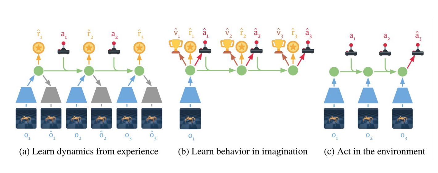
|
||||
|
||||
Representation model: $p_\theta(s_t|s_{t-1}, a_{t-1}, o_t)$
|
||||
|
||||
Observation model: $q_\theta(o_t|s_t)$
|
||||
|
||||
Reward model: $q_\theta(r_t|s_t)$
|
||||
|
||||
Transition model: $q_\theta(s_t| s_{t-1}, a_{t-1})$.
|
||||
|
||||
Variational evidence lower bound (ELBO) objective:
|
||||
|
||||
$$
|
||||
\mathcal{J}_{REC}\doteq \mathbb{E}_{p}\left(\sum_t(\mathcal{J}_O^t+\mathcal{J}_R^t+\mathcal{J}_D^t)\right)
|
||||
$$
|
||||
|
||||
where
|
||||
|
||||
$$
|
||||
\mathcal{J}_O^t\doteq \ln q(o_t|s_t)
|
||||
$$
|
||||
|
||||
$$
|
||||
\mathcal{J}_R^t\doteq \ln q(r_t|s_t)
|
||||
$$
|
||||
|
||||
$$
|
||||
\mathcal{J}_D^t\doteq -\beta \operatorname{KL}(p(s_t|s_{t-1}, a_{t-1}, o_t)||q(s_t|s_{t-1}, a_{t-1}))
|
||||
$$
|
||||
|
||||
#### More versions for Dreamer
|
||||
|
||||
Latest is V3, [link to the paper](https://arxiv.org/pdf/2301.04104)
|
||||
|
||||
### Learn in Latent Space
|
||||
|
||||
- Pros
|
||||
- Learn visual skill efficiently (using relative simple networks)
|
||||
- Cons
|
||||
- Using autoencoder might not recover the right representation
|
||||
- Not necessarily suitable for model-based methods
|
||||
- Embedding is often not a good state representation without using history observations
|
||||
|
||||
### Planning with Value Prediction Network (VPN)
|
||||
|
||||
Idea: generating trajectories by following $\epsilon$-greedy policy based on the planning method
|
||||
|
||||
Q-value calculated from $d$-step planning is defined as:
|
||||
|
||||
$$
|
||||
Q_\theta^d(s,o)=r+\gamma V_\theta^{d}(s')
|
||||
$$
|
||||
|
||||
$$
|
||||
V_\theta^{d}(s)=\begin{cases}
|
||||
V_\theta(s) & \text{if } d=1\\
|
||||
\frac{1}{d}V_\theta(s)+\frac{d-1}{d}\max_{o} Q_\theta^{d-1}(s,o)& \text{if } d>1
|
||||
\end{cases}
|
||||
$$
|
||||
|
||||
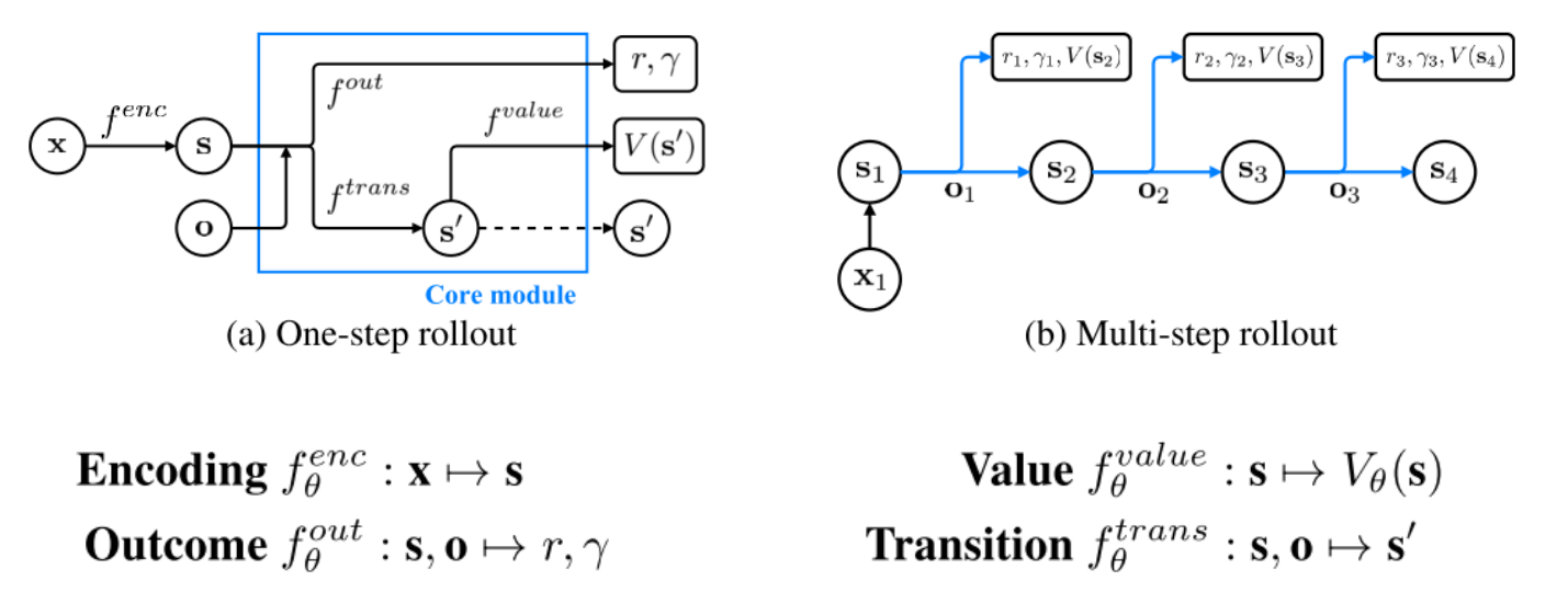
|
||||
|
||||
Given an n-step trajectory $x_1, o_1, r_1, \gamma_1, x_2, o_2, r_2, \gamma_2, ..., x_{n+1}$ generated by the $\epsilon$-greedy policy, k-step predictions are defined as follows:
|
||||
|
||||
$$
|
||||
s_t^k=\begin{cases}
|
||||
f^{enc}_\theta(x_t) & \text{if } k=0\\
|
||||
f^{trans}_\theta(s_{t-1}^{k-1},o_{t-1}) & \text{if } k>0
|
||||
\end{cases}
|
||||
$$
|
||||
|
||||
$$
|
||||
v_t^k=f^{value}_\theta(s_t^k)
|
||||
$$
|
||||
|
||||
$$
|
||||
r_t^k,\gamma_t^k=f^{out}_\theta(s_t^{k-1},o_t)
|
||||
$$
|
||||
|
||||
$$
|
||||
\mathcal{L}_t=\sum_{l=1}^k(R_t-v_t^l)^2+(r_t-r_t^l)^2+(\gamma_t-\gamma_t^l)^2\text{ where } R_t=\begin{cases}
|
||||
r_t+\gamma_t R_{t+1} & \text{if } t\leq n\\
|
||||
\max_{o} Q_{\theta-}^d(s_{n+1},o)& \text{if } t=n+1
|
||||
\end{cases}
|
||||
$$
|
||||
|
||||
### MuZero
|
||||
|
||||
beats AlphaZero
|
||||
@@ -1,187 +0,0 @@
|
||||
# CSE510 Deep Reinforcement Learning (Lecture 2)
|
||||
|
||||
Introduction and Markov Decision Processes (MDPs)
|
||||
|
||||
## What is reinforcement learning (RL)
|
||||
|
||||
- A general computational framework for behavior learning through reinforcement/trial and error
|
||||
- Deep RL: combining deep learning with RL for complex problems
|
||||
- Showing a promise for artificial general intelligence (AGI)
|
||||
|
||||
## What RL can do now.
|
||||
|
||||
### Backgammon
|
||||
|
||||
#### Neuro-Gammon
|
||||
|
||||
Developed by Gerald Tesauro in 1989 in IBM's research center.
|
||||
|
||||
Train to mimic expert demonstrations using supervised learning.
|
||||
|
||||
Achieved intermediate-level human player.
|
||||
|
||||
#### TD-Gammon (Temporal Difference Learning)
|
||||
|
||||
Developed by Gerald Tesauro in 1992 in IBM's research center.
|
||||
|
||||
A neural network that trains itself to be an evaluation function by playing against itself starting from random weights.
|
||||
|
||||
Achieved performance close to top human players of its time.
|
||||
|
||||
### DeepMind Atari
|
||||
|
||||
Use deep Q-learning to play Atari games.
|
||||
|
||||
Without human demonstrations, it can learn to play the game at a superhuman level.
|
||||
|
||||
### AlphaGo
|
||||
|
||||
Monte Carlo Tree Search, learning policy and value function networks for pruning the search tree, expert demonstrations, self-play, and TPU from Google.
|
||||
|
||||
### Video Games
|
||||
|
||||
OpenAI Five for Dota 2
|
||||
|
||||
won 5v5 best of 3 games against top human players.
|
||||
|
||||
Deepmind AlphaStar for StarCraft
|
||||
|
||||
supervised training followed by a league competition training.
|
||||
|
||||
### AlphaTensor
|
||||
|
||||
discovering faster matrix multiplication algorithms with reinforcement learning.
|
||||
|
||||
AlphaTensor: 76 vs Strassen's 80 for 5x5 matrix multiplication.
|
||||
|
||||
### Training LLMs
|
||||
|
||||
For verifiable tasks (coding, math, etc.), RL can be used to train a model to perform the task without human supervision.
|
||||
|
||||
### Robotics
|
||||
|
||||
Unitree Go, Altlas by Boston Dynamics, etc.
|
||||
|
||||
## What are the challenges of RL in real world applications?
|
||||
|
||||
Beating the human champion is "easier" than placing the go stones.
|
||||
|
||||
### State estimation
|
||||
|
||||
Known environments (known entities and dynamics) vs. unknown environments (unknown entities and dynamics).
|
||||
|
||||
Need for behaviors to **transfer/generalize** across environmental variations since the real world is very diverse.
|
||||
|
||||
> **State estimation**
|
||||
>
|
||||
> To be able to act, you need first to be able to **see**, detect the **objects** that you interact with, detect whether you achieved the **goal**.
|
||||
|
||||
Most works are between two extremes:
|
||||
|
||||
- Assuming the world model known (object locations, shapes, physical properties obtain via AR tags or manual tuning), they use planners to search for the action sequence to achieve a desired goal.
|
||||
|
||||
- Do not attempt to detect any objects and learn to map RGB images directly to actions.
|
||||
|
||||
Behavior learning is challenging because state estimation is challenging, in other word, because computer vision/perception is challenging.
|
||||
|
||||
Interesting direction: **leveraging DRL and vision-language models**
|
||||
|
||||
### Efficiency
|
||||
|
||||
Cheap vs. Expensive to get experience samples
|
||||
|
||||
#### DRL Sample Efficiency
|
||||
|
||||
Humans after 15 minutes tend to outperform DDQN after
|
||||
115 hours
|
||||
|
||||
#### Reinforcement Learning in Human
|
||||
|
||||
Human appear to learn to act (e.g., walk) through "very few examples" of trial and error. How is an open question...
|
||||
|
||||
Possible answers:
|
||||
|
||||
- Hardware: 230 million years of bipedal movement data
|
||||
- Imitation Learning: Observation of other humans walking (e.g., imitation learning, episodic memory and semantic memory)
|
||||
- Algorithms: Better than backpropagation and stochastic gradient descent
|
||||
|
||||
#### Discrete and continuous action spaces
|
||||
|
||||
Computation is discrete, but the real action space is continuous.
|
||||
|
||||
#### One-goal vs. Multi-goal
|
||||
|
||||
Life is a multi-goal problem. Involving infinitely many possible games.
|
||||
|
||||
#### Rewards automatic and auto detect rewards
|
||||
|
||||
Our curiosity is a reward.
|
||||
|
||||
#### And more
|
||||
|
||||
- Transfer learning
|
||||
- Generalization
|
||||
- Long horizon reasoning
|
||||
- Model-based RL
|
||||
- Sparse rewards
|
||||
- Reward design/learning
|
||||
- Planning/Learning
|
||||
- Lifelong learning
|
||||
- Safety
|
||||
- Interpretability
|
||||
- etc.
|
||||
|
||||
## What is the course about?
|
||||
|
||||
To teach you RL models and algorithms.
|
||||
|
||||
- To be able to tackle real world problems.
|
||||
|
||||
To excite you about RL.
|
||||
|
||||
- To provide a primer for you to launch advanced studies.
|
||||
|
||||
Schedule:
|
||||
|
||||
- RL Model and basic algorithms
|
||||
- Markov Decision Process (MDP)
|
||||
- Passive RL: ADP and TD-learning
|
||||
- Active RL: Q-Learning and SARSA
|
||||
- Deep RL algorithms
|
||||
- Value-Based methods
|
||||
- Policy Gradient Methods
|
||||
- Model-Based methods
|
||||
- Advanced Topics
|
||||
- Offline RL, Multi-Agent RL, etc.
|
||||
|
||||
### Reinforcement Learning Algorithms
|
||||
|
||||
#### Model-Based
|
||||
|
||||
- Learn the model of the world, then plan using the model
|
||||
- Update model often
|
||||
- Re-plan often
|
||||
|
||||
#### Value-Based
|
||||
|
||||
- Learn the state or state-action value
|
||||
- Act by choosing best action in state
|
||||
- Exploration is a necessary add-on
|
||||
|
||||
#### Policy-based
|
||||
|
||||
- Learn the stochastic policy function that maps state to action
|
||||
- Act by sampling policy
|
||||
- Exploration is baked in
|
||||
|
||||
#### Better sample efficiency to Less sample efficiency
|
||||
|
||||
- Model-Based
|
||||
- Off-policy/Q-learning
|
||||
- Actor-critic
|
||||
- On-policy/Policy gradient
|
||||
- Evolutionary/Gradient-free
|
||||
|
||||
## What is RL?
|
||||
|
||||
## RL model: Markov Decision Process (MDP)
|
||||
@@ -1,143 +0,0 @@
|
||||
# CSE510 Deep Reinforcement Learning (Lecture 20)
|
||||
|
||||
## Exploration in RL
|
||||
|
||||
### Motivations
|
||||
|
||||
#### Exploration vs. Exploitation Dilemma
|
||||
|
||||
Online decision-making involves a fundamental choice:
|
||||
|
||||
- Exploration: trying out new things (new behaviors), with the hope of discovering higher rewards
|
||||
- Exploitation: doing what you know will yield the highest reward
|
||||
|
||||
The best long-term strategy may involve short-term sacrifices
|
||||
|
||||
Gather enough knowledge early to make the best long-term decisions
|
||||
|
||||
<details>
|
||||
<summary>Example</summary>
|
||||
Restaurant Selection
|
||||
|
||||
- Exploitation: Go to your favorite restaurant
|
||||
- Exploration: Try a new restaurant
|
||||
|
||||
Oil Drilling
|
||||
|
||||
- Exploitation: Drill at the best known location
|
||||
- Exploration: Drill at a new location
|
||||
|
||||
Game Playing
|
||||
|
||||
- Exploitation: Play the move you believe is best
|
||||
- Exploration: Play an experimental move
|
||||
|
||||
</details>
|
||||
|
||||
#### Breakout vs. Montezuma's Revenge
|
||||
|
||||
| Property | Breakout | Montezuma's Revenge |
|
||||
|----------|----------|--------------------|
|
||||
| **Reward frequency** | Dense (every brick hit gives points) | Extremely sparse (only after collecting key or treasure) |
|
||||
| **State space** | Simple (ball, paddle, bricks) | Complex (many rooms, objects, ladders, timing) |
|
||||
| **Action relevance** | Almost any action affects reward soon | Most actions have no immediate feedback |
|
||||
| **Exploration depth** | Shallow (few steps to reward) | Deep (dozens/hundreds of steps before reward) |
|
||||
| **Determinism** | Mostly deterministic dynamics | Deterministic but requires long sequences of precise actions |
|
||||
| **Credit assignment** | Easy — short time gap | Very hard — long delay from cause to effect |
|
||||
|
||||
#### Motivation
|
||||
|
||||
- Motivation: "Forces" that energize an organism to act and that direct its activity
|
||||
- Extrinsic Motivation: being motivated to do something because of some external reward ($, a prize, food, water, etc.)
|
||||
- Intrinsic Motivation: being motivated to do something because it is inherently enjoyable (curiosity, exploration, novelty, surprise, incongruity, complexity…)
|
||||
|
||||
### Intuitive Exploration Strategy
|
||||
|
||||
- Intrinsic motivation drives the exploration for unknowns
|
||||
- Intuitively, we explore efficiently once we know what we do not know, and target our exploration efforts to the unknown part of the space.
|
||||
- All non-naive exploration methods consider some form of uncertainty estimation, regarding state (or state-action) I have visited, transition dynamics, or Q-functions.
|
||||
|
||||
- Optimal methods in smaller settings don't work, but can inspire for larger settings
|
||||
- May use some hacks
|
||||
|
||||
### Classes of Exploration Methods in Deep RL
|
||||
|
||||
- Optimistic exploration
|
||||
- Uncertainty about states
|
||||
- Visiting novel states (state visitation counting)
|
||||
- Information state search
|
||||
- Uncertainty about state transitions or dynamics
|
||||
- Dynamics prediction error or Information gain for dynamics learning
|
||||
- Posterior sampling
|
||||
- Uncertainty about Q-value functions or policies
|
||||
- Selecting actions according to the probability they are best
|
||||
|
||||
### Optimistic Exploration
|
||||
|
||||
#### Count-Based Exploration in Small MDPs
|
||||
|
||||
Book-keep state visitation counts $N(s)$
|
||||
Add exploration reward bonuses that encourage policies that visit states with fewer counts.
|
||||
|
||||
$$
|
||||
R(s,a,s') = r(s,a,s') + \mathcal{B}(N(s))
|
||||
$$
|
||||
|
||||
where $\mathcal{B}(N(s))$ is the intrinsic exploration reward bonus.
|
||||
|
||||
- UCB: $\mathcal{B}(N(s)) = \sqrt{\frac{2\ln n}{N(s)}}$ (more aggressive exploration)
|
||||
- MBIE-EB (Strehl & Littman): $\mathcal{B}(N(s)) = \sqrt{\frac{1}{N(s)}}$
|
||||
- BEB (Kolter & Ng): $\mathcal{B}(N(s)) = \frac{1}{N(s)}$
|
||||
|
||||
- We want to come up with something that rewards states that we have not visited often.
|
||||
- But in large MDPs, we rarely visit a state twice!
|
||||
- We need to capture a notion of state similarity, and reward states that are most dissimilar to what we have seen so far
|
||||
- as opposed to different (as they will always be different).
|
||||
|
||||
#### Fitting Generative Models
|
||||
|
||||
Idea: fit a density model $p_\theta(s)$ (or $p_\theta(s,a)$)
|
||||
|
||||
$p_\theta(s)$ might be high even for a new $s$.
|
||||
|
||||
If $s$ is similar to perviously seen states, can we use $p_\theta(s)$ to get a "pseudo-count" for $s$?
|
||||
|
||||
If we have small MDPs, the true probability is
|
||||
|
||||
$$
|
||||
P(s)=\frac{N(s)}{n}
|
||||
$$
|
||||
|
||||
where $N(s)$ is the number of times $s$ has been visited and $n$ is the total states visited.
|
||||
|
||||
after we visit $s$, then
|
||||
|
||||
$$
|
||||
P'(s)=\frac{N(s)+1}{n+1}
|
||||
$$
|
||||
|
||||
1. fit model $p_\theta(s)$ to all states $\mathcal{D}$ so far.
|
||||
2. take a step $i$ and observe $s_i$.
|
||||
3. fit new model $p_\theta'(s)$ to all states $\mathcal{D} \cup {s_i}$.
|
||||
4. use $p_\theta(s_i)$ and $p_\theta'(s_i)$ to estimate the "pseudo-count" for $\hat{N}(s_i)$.
|
||||
5. set $r_i^+=r_i+\mathcal{B}(\hat{N}(s_i))$
|
||||
6. go to 1
|
||||
|
||||
How to get $\hat{N}(s_i)$? use the equations
|
||||
|
||||
$$
|
||||
p_\theta(s_i)=\frac{\hat{N}(s_i)}{\hat{n}}\quad p_\theta'(s_i)=\frac{\hat{N}(s_i)+1}{\hat{n}+1}
|
||||
$$
|
||||
|
||||
[link to the paper](https://arxiv.org/pdf/1606.01868)
|
||||
|
||||
#### Density models
|
||||
|
||||
[link to the paper](https://arxiv.org/pdf/1703.01310)
|
||||
|
||||
#### State Counting with DeepHashing
|
||||
|
||||
- We still count states (images) but not in pixel space, but in latent compressed space.
|
||||
- Compress $s$ into a latent code, then count occurrences of the code.
|
||||
- How do we get the image encoding? e.g., using autoencoders.
|
||||
- There is no guarantee such reconstruction loss will capture the important things that make two states to be similar
|
||||
@@ -1,242 +0,0 @@
|
||||
# CSE510 Deep Reinforcement Learning (Lecture 21)
|
||||
|
||||
> Due to lack of my attention, this lecture note is generated by ChatGPT to create continuations of the previous lecture note.
|
||||
|
||||
## Exploration in RL: Information-Based Exploration (Intrinsic Curiosity)
|
||||
|
||||
### Computational Curiosity
|
||||
|
||||
- "The direct goal of curiosity and boredom is to improve the world model."
|
||||
- Curiosity encourages agents to seek experiences that better predict or explain the environment.
|
||||
- A "curiosity unit" gives reward based on the mismatch between current model predictions and actual outcomes.
|
||||
- Intrinsic reward is high when the agent's prediction fails, that is, when it encounters surprising outcomes.
|
||||
- This yields positive intrinsic reinforcement when the internal predictive model errs, causing the agent to repeat actions that lead to prediction errors.
|
||||
- The agent is effectively motivated to create situations where its model fails.
|
||||
|
||||
### Model Prediction Error as Intrinsic Reward
|
||||
|
||||
We augment the reward with an intrinsic bonus based on model prediction error:
|
||||
|
||||
$R(s, a, s') = r(s, a, s') + B(|T(s, a; \theta) - s'|)$
|
||||
|
||||
Parameter explanations:
|
||||
|
||||
- $s$: current state of the agent.
|
||||
- $a$: action taken by the agent in state $s$.
|
||||
- $s'$: next state resulting from executing action $a$ in state $s$.
|
||||
- $r(s, a, s')$: extrinsic environment reward for transition $(s, a, s')$.
|
||||
- $T(s, a; \theta)$: learned dynamics model with parameters $\theta$ that predicts the next state.
|
||||
- $\theta$: parameter vector of the predictive dynamics model $T$.
|
||||
- $|T(s, a; \theta) - s'|$: prediction error magnitude between predicted next state and actual next state.
|
||||
- $B(\cdot)$: function converting prediction error magnitude into an intrinsic reward bonus.
|
||||
- $R(s, a, s')$: total reward, sum of extrinsic reward and intrinsic curiosity bonus.
|
||||
|
||||
Key ideas:
|
||||
|
||||
- The agent receives an intrinsic reward $B(|T(s, a; \theta) - s'|)$ when the actual outcome differs from what its world model predicts.
|
||||
- Initially many transitions are surprising, encouraging broad exploration.
|
||||
- As the model improves, familiar transitions yield smaller error and smaller intrinsic reward.
|
||||
- Exploration becomes focused on less-known parts of the state space.
|
||||
- Intrinsic motivation is non-stationary: as the agent learns, previously novel states lose their intrinsic reward.
|
||||
|
||||
#### Avoiding Trivial Curiosity Traps
|
||||
|
||||
[link to paper](https://ar5iv.labs.arxiv.org/html/1705.05363#:~:text=reward%20signal%20based%20on%20how,this%20feature%20space%20using%20self)
|
||||
|
||||
Naively defining $B(s, a, s')$ directly in raw observation space can lead to trivial curiosity traps.
|
||||
|
||||
Examples:
|
||||
|
||||
- The agent may purposely cause chaotic or noisy observations (like flickering pixels) that are impossible to predict.
|
||||
- The model cannot reduce prediction error on pure noise, so the agent is rewarded for meaningless randomness.
|
||||
- This yields high intrinsic reward without meaningful learning or progress toward task goals.
|
||||
|
||||
To prevent this, we restrict prediction to a more informative feature space:
|
||||
|
||||
$B(s, a, s') = |T(E(s; \phi), a; \theta) - E(s'; \phi)|$
|
||||
|
||||
Parameter explanations:
|
||||
|
||||
- $E(s; \phi)$: learned encoder mapping raw state $s$ into a feature vector.
|
||||
- $\phi$: parameter vector of the encoder $E$.
|
||||
- $T(E(s; \phi), a; \theta)$: forward model predicting next feature representation from encoded state and action.
|
||||
- $E(s'; \phi)$: encoded feature representation of the next state $s'$.
|
||||
- $B(s, a, s')$: intrinsic reward based on prediction error in feature space.
|
||||
|
||||
Key ideas:
|
||||
|
||||
- The encoder $E(s; \phi)$ is trained so that features capture aspects of the state that are controllable by the agent.
|
||||
- One approach is to train $E$ via an inverse dynamics model that predicts $a$ from $(s, s')$.
|
||||
- This encourages $E$ to keep only information necessary to infer actions, discarding irrelevant noise.
|
||||
- Measuring prediction error in feature space ignores unpredictable environmental noise.
|
||||
- Intrinsic reward focuses on errors due to lack of knowledge about controllable dynamics.
|
||||
- The agent's curiosity is directed toward aspects of the environment it can influence and learn.
|
||||
|
||||
A practical implementation is the Intrinsic Curiosity Module (ICM) by Pathak et al. (2017):
|
||||
|
||||
- The encoder $E$ and forward model $T$ are trained jointly.
|
||||
- The loss includes both forward prediction error and inverse dynamics error.
|
||||
- Intrinsic reward is set to the forward prediction error in feature space.
|
||||
- This drives exploration of states where the agent cannot yet predict the effect of its actions.
|
||||
|
||||
#### Random Network Distillation (RND)
|
||||
|
||||
Random Network Distillation (RND) provides a simpler curiosity bonus without learning a dynamics model.
|
||||
|
||||
Basic idea:
|
||||
|
||||
- Use a fixed random neural network $f_{\text{target}}$ that maps states to feature vectors.
|
||||
- Train a predictor network $f_{\text{pred}}$ to approximate $f_{\text{target}}$ on visited states.
|
||||
- The intrinsic reward is the prediction error between $f_{\text{pred}}(s)$ and $f_{\text{target}}(s)$.
|
||||
|
||||
Typical form of the intrinsic reward:
|
||||
|
||||
$r^{\text{int}}(s) = |f_{\text{pred}}(s; \psi) - f_{\text{target}}(s)|^{2}$
|
||||
|
||||
Parameter explanations:
|
||||
|
||||
- $f_{\text{target}}$: fixed random neural network generating target features for each state.
|
||||
- $f_{\text{pred}}(s; \psi)$: trainable predictor network with parameters $\psi$.
|
||||
- $\psi$: parameter vector for the predictor network.
|
||||
- $s$: state input to both networks.
|
||||
- $|f_{\text{pred}}(s; \psi) - f_{\text{target}}(s)|^{2}$: squared error between predictor and target features.
|
||||
- $r^{\text{int}}(s)$: intrinsic reward based on prediction error in random feature space.
|
||||
|
||||
Key properties:
|
||||
|
||||
- For novel or rarely visited states, $f_{\text{pred}}$ has not yet learned to match $f_{\text{target}}$, so error is high.
|
||||
- For frequently visited states, prediction error becomes small, and intrinsic reward decays.
|
||||
- The target network is random and fixed, so it does not adapt to the policy.
|
||||
- This provides a stable novelty signal without explicit dynamics learning.
|
||||
- RND achieves strong exploration performance in challenging environments, such as hard-exploration Atari games.
|
||||
|
||||
### Efficacy of Curiosity-Driven Exploration
|
||||
|
||||
Empirical observations:
|
||||
|
||||
- Curiosity-driven intrinsic rewards often lead to significantly higher extrinsic returns in sparse-reward environments compared to agents trained only on extrinsic rewards.
|
||||
- Intrinsic rewards act as a proxy objective that guides the agent toward interesting or informative regions of the state space.
|
||||
- In some experiments, agents trained with only intrinsic rewards (no extrinsic reward during training) still learn behaviors that later achieve high task scores when extrinsic rewards are measured.
|
||||
- Using random features for curiosity (as in RND) can perform nearly as well as using learned features in many domains.
|
||||
- Simple surprise signals are often sufficient to drive effective exploration.
|
||||
- Learned feature spaces may generalize better to truly novel scenarios but are not always necessary.
|
||||
|
||||
Historical context:
|
||||
|
||||
- The concept of learning from intrinsic rewards alone is not new.
|
||||
- Itti and Baldi (2005) studied "Bayesian surprise" as a driver of human attention.
|
||||
- Schmidhuber (1991, 2010) formalized curiosity, creativity, and fun as intrinsic motivations in learning agents.
|
||||
- Singh et al. (2004) proposed intrinsically motivated reinforcement learning frameworks.
|
||||
- These early works laid the conceptual foundation for modern curiosity-driven deep RL methods.
|
||||
|
||||
For further reading on intrinsic curiosity methods:
|
||||
|
||||
- Pathak et al., "Curiosity-driven Exploration by Self-supervised Prediction", 2017.
|
||||
- Burda et al., "Exploration by Random Network Distillation", 2018.
|
||||
- Schmidhuber, "Formal Theory of Creativity, Fun, and Intrinsic Motivation", 2010.
|
||||
|
||||
## Exploration via Posterior Sampling
|
||||
|
||||
While optimistic and curiosity bonus methods modify the reward function, posterior sampling approaches handle exploration by maintaining uncertainty over models or value functions and sampling from this uncertainty.
|
||||
|
||||
These methods are rooted in Thompson Sampling and naturally balance exploration and exploitation.
|
||||
|
||||
### Posterior Sampling in Multi-Armed Bandits (Thompson Sampling)
|
||||
|
||||
In a multi-armed bandit problem (no state transitions), Thompson Sampling works as follows:
|
||||
|
||||
1. Maintain a prior and posterior distribution over the reward parameters for each arm.
|
||||
2. At each time step, sample reward parameters for all arms from their current posterior.
|
||||
3. Select the arm with the highest sampled mean reward.
|
||||
4. Observe the reward, update the posterior, and repeat.
|
||||
|
||||
Intuition:
|
||||
|
||||
- Each action is selected with probability equal to the posterior probability that it is optimal.
|
||||
- Arms with high uncertainty are more likely to be sampled as optimal in some posterior draws.
|
||||
- Exploration arises naturally from uncertainty, without explicit epsilon-greedy noise or bonus terms.
|
||||
- Over time, the posterior concentrates on the true reward means, and the algorithm shifts toward exploitation.
|
||||
|
||||
Theoretical properties:
|
||||
|
||||
- Thompson Sampling attains near-optimal regret bounds in many bandit settings.
|
||||
- It often performs as well as or better than upper confidence bound algorithms in practice.
|
||||
|
||||
### Posterior Sampling for Reinforcement Learning (PSRL)
|
||||
|
||||
In reinforcement learning with states and transitions, posterior sampling generalizes to sampling entire MDP models.
|
||||
|
||||
Posterior Sampling for Reinforcement Learning (PSRL) operates as follows:
|
||||
|
||||
1. Maintain a posterior distribution over environment dynamics and rewards, based on observed transitions.
|
||||
2. At the beginning of an episode, sample an MDP model from this posterior.
|
||||
3. Compute the optimal policy for the sampled MDP (for example, by value iteration).
|
||||
4. Execute this policy in the real environment for the whole episode.
|
||||
5. Use the observed transitions to update the posterior, then repeat.
|
||||
|
||||
Key advantages:
|
||||
|
||||
- The agent commits to a sampled model's policy for an extended duration, which induces deep exploration.
|
||||
- If a sampled model is optimistic in unexplored regions, the corresponding policy will deliberately visit those regions.
|
||||
- Exploration is coherent across time within an episode, unlike per-step randomization in epsilon-greedy.
|
||||
- The method does not require ad hoc exploration bonuses; exploration is an emergent property of the posterior.
|
||||
|
||||
Challenges:
|
||||
|
||||
- Maintaining an exact posterior over high-dimensional MDPs is usually intractable.
|
||||
- Practical implementations use approximations.
|
||||
|
||||
### Approximate Posterior Sampling with Ensembles (Bootstrapped DQN)
|
||||
|
||||
A common approximate posterior method in deep RL is Bootstrapped DQN.
|
||||
|
||||
Basic idea:
|
||||
|
||||
- Train an ensemble of $K$ Q-networks (heads), $Q^{(1)}, \dots, Q^{(K)}$.
|
||||
- Each head is trained on a different bootstrap sample or masked subset of experience.
|
||||
- At the start of each episode, sample a head index $k$ uniformly from ${1, \dots, K}$.
|
||||
- For the entire episode, act greedily with respect to $Q^{(k)}$.
|
||||
|
||||
Parameter definitions for the ensemble:
|
||||
|
||||
- $K$: number of Q-network heads in the ensemble.
|
||||
- $Q^{(k)}(s, a)$: Q-value estimate for head $k$ at state-action pair $(s, a)$.
|
||||
- $k$: index of the sampled head used for the current episode.
|
||||
- $(s, a)$: state and action arguments to Q-value functions.
|
||||
|
||||
Implementation details:
|
||||
|
||||
- A shared feature backbone network processes state inputs, feeding into all heads.
|
||||
- Each head has its own final layers, allowing diverse value estimates.
|
||||
- Masking or bootstrapping assigns different subsets of transitions to different heads during training.
|
||||
|
||||
Benefits:
|
||||
|
||||
- Each head approximates a different plausible Q-function, analogous to a sample from a posterior.
|
||||
- When a head is optimistic about certain under-explored actions, its greedy policy will explore them deeply.
|
||||
- Exploration behavior is temporally consistent within an episode.
|
||||
- No modification of the reward function is required; exploration arises from policy randomization via multiple heads.
|
||||
|
||||
Comparison to epsilon-greedy:
|
||||
|
||||
- Epsilon-greedy adds per-step random actions, which can be inefficient for long-horizon exploration.
|
||||
- Bootstrapped DQN commits to a strategy for an episode, enabling the agent to execute complete exploratory plans.
|
||||
- This can dramatically increase the probability of discovering long sequences needed to reach sparse rewards.
|
||||
|
||||
Other approximate posterior approaches:
|
||||
|
||||
- Bayesian neural networks for Q-functions (explicit parameter distributions).
|
||||
- Using Monte Carlo dropout at inference to sample Q-functions.
|
||||
- Randomized prior functions added to Q-networks to maintain exploration.
|
||||
|
||||
Theoretical insights:
|
||||
|
||||
- Posterior sampling methods can enjoy strong regret bounds in some RL settings.
|
||||
- They can have better asymptotic constants than optimism-based methods in certain problems.
|
||||
- Coherent, temporally extended exploration is essential in environments with delayed rewards and complex goals.
|
||||
|
||||
For further reading:
|
||||
|
||||
- Osband et al., "Deep Exploration via Bootstrapped DQN", 2016.
|
||||
- Osband and Van Roy, "Why Is Posterior Sampling Better Than Optimism for Reinforcement Learning?", 2017.
|
||||
- Chapelle and Li, "An Empirical Evaluation of Thompson Sampling", 2011.
|
||||
@@ -1,296 +0,0 @@
|
||||
# CSE510 Deep Reinforcement Learning (Lecture 22)
|
||||
|
||||
> Due to lack of my attention, this lecture note is generated by ChatGPT to create continuations of the previous lecture note.
|
||||
|
||||
## Offline Reinforcement Learning: Introduction and Challenges
|
||||
|
||||
Offline reinforcement learning (offline RL), also called batch RL, aims to learn an optimal policy -without- interacting with the environment. Instead, the agent is given a fixed dataset of transitions collected by an unknown behavior policy.
|
||||
|
||||
### The Offline RL Dataset
|
||||
|
||||
We are given a static dataset:
|
||||
|
||||
$$
|
||||
D = { (s_i, a_i, s'-i, r_i ) }-{i=1}^N
|
||||
$$
|
||||
|
||||
Parameter explanations:
|
||||
|
||||
- $s_i$: state sampled from behavior policy state distribution.
|
||||
- $a_i$: action selected by the behavior policy $\pi_beta$.
|
||||
- $s'_i$: next state sampled from environment dynamics $p(s'|s,a)$.
|
||||
- $r_i$: reward observed for transition $(s_i,a_i)$.
|
||||
- $N$: total number of transitions in the dataset.
|
||||
- $D$: full offline dataset used for training.
|
||||
|
||||
The goal is to learn a new policy $\pi$ maximizing expected discounted return using only $D$:
|
||||
|
||||
$$
|
||||
\max_{\pi} ; \mathbb{E}\Big[\sum_{t=0}^T \gamma^t r(s_t, a_t)\Big]
|
||||
$$
|
||||
|
||||
Parameter explanations:
|
||||
|
||||
- $\pi$: policy we want to learn.
|
||||
- $r(s,a)$: reward received for state-action pair.
|
||||
- $\gamma$: discount factor controlling weight of future rewards.
|
||||
- $T$: horizon or trajectory length.
|
||||
|
||||
### Why Offline RL Is Difficult
|
||||
|
||||
Offline RL is fundamentally harder than online RL because:
|
||||
|
||||
- The agent cannot try new actions to fix wrong value estimates.
|
||||
- The policy may choose out-of-distribution actions not present in $D$.
|
||||
- Q-value estimates for unseen actions can be arbitrarily incorrect.
|
||||
- Bootstrapping on wrong Q-values can cause divergence.
|
||||
|
||||
This leads to two major failure modes:
|
||||
|
||||
1. --Distribution shift--: new policy actions differ from dataset actions.
|
||||
2. --Extrapolation error--: the Q-function guesses values for unseen actions.
|
||||
|
||||
### Extrapolation Error Problem
|
||||
|
||||
In standard Q-learning, the Bellman backup is:
|
||||
|
||||
$$
|
||||
Q(s,a) \leftarrow r + \gamma \max_{a'} Q(s', a')
|
||||
$$
|
||||
|
||||
Parameter explanations:
|
||||
|
||||
- $Q(s,a)$: estimated value of taking action $a$ in state $s$.
|
||||
- $\max_{a'}$: maximum over possible next actions.
|
||||
- $a'$: candidate next action for evaluation in backup step.
|
||||
|
||||
If $a'$ was rarely or never taken in the dataset, $Q(s',a')$ is poorly estimated, so Q-learning boots off invalid values, causing instability.
|
||||
|
||||
### Behavior Cloning (BC): The Safest Baseline
|
||||
|
||||
The simplest offline method is to imitate the behavior policy:
|
||||
|
||||
$$
|
||||
\max_{\phi} ; \mathbb{E}_{(s,a) \sim D}[\log \pi_{\phi}(a|s)]
|
||||
$$
|
||||
|
||||
Parameter explanations:
|
||||
|
||||
- $\phi$: neural network parameters of the cloned policy.
|
||||
- $\pi_{\phi}$: learned policy approximating behavior policy.
|
||||
- $\log \pi_{\phi}(a|s)$: negative log-likelihood loss.
|
||||
|
||||
Pros:
|
||||
|
||||
- Does not suffer from extrapolation error.
|
||||
- Extremely stable.
|
||||
|
||||
Cons:
|
||||
|
||||
- Cannot outperform the behavior policy.
|
||||
- Ignores reward information entirely.
|
||||
|
||||
### Naive Offline Q-Learning Fails
|
||||
|
||||
Directly applying off-policy Q-learning on $D$ generally leads to:
|
||||
|
||||
- Overestimation of unseen actions.
|
||||
- Divergence due to extrapolation error.
|
||||
- Policies worse than behavior cloning.
|
||||
|
||||
## Strategies for Safe Offline RL
|
||||
|
||||
There are two primary families of solutions:
|
||||
|
||||
1. --Policy constraint methods--
|
||||
2. --Conservative value estimation methods--
|
||||
|
||||
## 1. Policy Constraint Methods
|
||||
|
||||
These methods restrict the learned policy to stay close to the behavior policy so it does not take unsupported actions.
|
||||
|
||||
### Advantage Weighted Regression (AWR / AWAC)
|
||||
|
||||
Policy update:
|
||||
|
||||
$$
|
||||
\pi(a|s) \propto \pi_{beta}(a|s)\exp\left(\frac{1}{\lambda}A(s,a)\right)
|
||||
$$
|
||||
|
||||
Parameter explanations:
|
||||
|
||||
- $\pi_{beta}$: behavior policy used to collect dataset.
|
||||
- $A(s,a)$: advantage function derived from Q or V estimates.
|
||||
- $\lambda$: temperature controlling strength of advantage weighting.
|
||||
- $\exp(\cdot)$: positive weighting on high-advantage actions.
|
||||
|
||||
Properties:
|
||||
|
||||
- Uses advantages to filter good and bad actions.
|
||||
- Improves beyond behavior policy while staying safe.
|
||||
|
||||
### Batch-Constrained Q-learning (BCQ)
|
||||
|
||||
BCQ constrains the policy using a generative model:
|
||||
|
||||
1. Train a VAE $G_{\omega}$ to model $a$ given $s$.
|
||||
2. Train a small perturbation model $\xi$.
|
||||
3. Limit the policy to $a = G_{\omega}(s) + \xi(s)$.
|
||||
|
||||
Parameter explanations:
|
||||
|
||||
- $G_{\omega}(s)$: VAE-generated action similar to data actions.
|
||||
- $\omega$: VAE parameters.
|
||||
- $\xi(s)$: small correction to generated actions.
|
||||
- $a$: final policy action constrained near dataset distribution.
|
||||
|
||||
BCQ avoids selecting unseen actions and strongly reduces extrapolation.
|
||||
|
||||
### BEAR (Bootstrapping Error Accumulation Reduction)
|
||||
|
||||
BEAR adds explicit constraints:
|
||||
|
||||
$$
|
||||
D_{MMD}\left(\pi(a|s), \pi_{beta}(a|s)\right) < \epsilon
|
||||
$$
|
||||
|
||||
Parameter explanations:
|
||||
|
||||
- $D_{MMD}$: Maximum Mean Discrepancy distance between action distributions.
|
||||
- $\epsilon$: threshold restricting policy deviation from behavior policy.
|
||||
|
||||
BEAR controls distribution shift more tightly than BCQ.
|
||||
|
||||
## 2. Conservative Value Function Methods
|
||||
|
||||
These methods modify Q-learning so Q-values of unseen actions are -underestimated-, preventing the policy from exploiting overestimated values.
|
||||
|
||||
### Conservative Q-Learning (CQL)
|
||||
|
||||
One formulation is:
|
||||
|
||||
$$
|
||||
J(Q) = J_{TD}(Q) + \alpha\big(\mathbb{E}_{a\sim\pi(\cdot|s)}Q(s,a) - \mathbb{E}_{a\sim D}Q(s,a)\big)
|
||||
$$
|
||||
|
||||
Parameter explanations:
|
||||
|
||||
- $J_{TD}$: standard Bellman TD loss.
|
||||
- $\alpha$: weight of conservatism penalty.
|
||||
- $\mathbb{E}_{a\sim\pi(\cdot|s)}$: expectation over policy-chosen actions.
|
||||
- $\mathbb{E}_{a\sim D}$: expectation over dataset actions.
|
||||
|
||||
Effect:
|
||||
|
||||
- Increases Q-values of dataset actions.
|
||||
- Decreases Q-values of out-of-distribution actions.
|
||||
|
||||
### Implicit Q-Learning (IQL)
|
||||
|
||||
IQL avoids constraints entirely by using expectile regression:
|
||||
|
||||
Value regression:
|
||||
|
||||
$$
|
||||
V(s) = \arg\min_{v} ; \mathbb{E}\big[\rho_{\tau}(Q(s,a) - v)\big]
|
||||
$$
|
||||
|
||||
Parameter explanations:
|
||||
|
||||
- $v$: scalar value estimate for state $s$.
|
||||
- $\rho_{\tau}(x)$: expectile regression loss.
|
||||
- $\tau$: expectile parameter controlling conservatism.
|
||||
- $Q(s,a)$: Q-value estimate.
|
||||
|
||||
Key idea:
|
||||
|
||||
- For $\tau < 1$, IQL reduces sensitivity to large (possibly incorrect) Q-values.
|
||||
- Implicitly conservative without special constraints.
|
||||
|
||||
IQL often achieves state-of-the-art performance due to simplicity and stability.
|
||||
|
||||
## Model-Based Offline RL
|
||||
|
||||
### Forward Model-Based RL
|
||||
|
||||
Train a dynamics model:
|
||||
|
||||
$$
|
||||
p_{\theta}(s'|s,a)
|
||||
$$
|
||||
|
||||
Parameter explanations:
|
||||
|
||||
- $p_{\theta}$: learned transition model.
|
||||
- $\theta$: parameters of transition model.
|
||||
|
||||
We can generate synthetic transitions using $p_{\theta}$, but model error accumulates.
|
||||
|
||||
### Penalty-Based Model Approaches (MOPO, MOReL)
|
||||
|
||||
Add uncertainty penalty:
|
||||
|
||||
$$
|
||||
r_{model}(s,a) = r(s,a) - \beta , u(s,a)
|
||||
$$
|
||||
|
||||
Parameter explanations:
|
||||
|
||||
- $r_{model}$: penalized reward for model rollouts.
|
||||
- $u(s,a)$: model uncertainty estimate.
|
||||
- $\beta$: penalty coefficient.
|
||||
|
||||
These methods limit exploration into unknown model regions.
|
||||
|
||||
## Reverse Model-Based Imagination (ROMI)
|
||||
|
||||
ROMI generates new training data by -backward- imagination.
|
||||
|
||||
### Reverse Dynamics Model
|
||||
|
||||
ROMI learns:
|
||||
|
||||
$$
|
||||
p_{\psi}(s_{t} \mid s_{t+1}, a_{t})
|
||||
$$
|
||||
|
||||
Parameter explanations:
|
||||
|
||||
- $\psi$: parameters of reverse dynamics model.
|
||||
- $s_{t+1}$: later state.
|
||||
- $a_{t}$: action taken leading to $s_{t+1}$.
|
||||
- $s_{t}$: predicted predecessor state.
|
||||
|
||||
ROMI also learns a reverse policy for sampling likely predecessor actions.
|
||||
|
||||
### Reverse Imagination Process
|
||||
|
||||
Given a goal state $s_{g}$:
|
||||
|
||||
1. Sample $a_{t}$ from reverse policy.
|
||||
2. Predict $s_{t}$ from reverse dynamics.
|
||||
3. Form imagined transition $(s_{t}, a_{t}, s_{t+1})$.
|
||||
4. Repeat to build longer imagined trajectories.
|
||||
|
||||
Benefits:
|
||||
|
||||
- Imagined transitions end in real states, ensuring grounding.
|
||||
- Completes missing parts of dataset.
|
||||
- Helps propagate reward backward reliably.
|
||||
|
||||
ROMI combined with conservative RL often outperforms standard offline methods.
|
||||
|
||||
# Summary of Lecture 22
|
||||
|
||||
Offline RL requires balancing:
|
||||
|
||||
- Improvement beyond dataset behavior.
|
||||
- Avoiding unsafe extrapolation to unseen actions.
|
||||
|
||||
Three major families of solutions:
|
||||
|
||||
1. Policy constraints (BCQ, BEAR, AWR)
|
||||
2. Conservative Q-learning (CQL, IQL)
|
||||
3. Model-based conservatism and imagination (MOPO, MOReL, ROMI)
|
||||
|
||||
Offline RL is becoming practical for real-world domains such as healthcare, robotics, autonomous driving, and recommender systems.
|
||||
@@ -1,162 +0,0 @@
|
||||
# CSE510 Deep Reinforcement Learning (Lecture 23)
|
||||
|
||||
> Due to lack of my attention, this lecture note is generated by ChatGPT to create continuations of the previous lecture note.
|
||||
|
||||
## Offline Reinforcement Learning Part II: Advanced Approaches
|
||||
|
||||
Lecture 23 continues with advanced topics in offline RL, expanding on model-based imagination methods and credit assignment structures relevant for offline multi-agent and single-agent settings.
|
||||
|
||||
## Reverse Model-Based Imagination (ROMI)
|
||||
|
||||
ROMI is a method for augmenting an offline dataset with additional transitions generated by imagining trajectories -backwards- from desirable states. Unlike forward model rollouts, backward imagination stays grounded in real data because imagined transitions always terminate in dataset states.
|
||||
|
||||
### Reverse Dynamics Model
|
||||
|
||||
ROMI learns a reverse dynamics model:
|
||||
|
||||
$$
|
||||
p_{\psi}(s_{t} \mid s_{t+1}, a_{t})
|
||||
$$
|
||||
|
||||
Parameter explanations:
|
||||
|
||||
- $p_{\psi}$: learned reverse transition model.
|
||||
- $\psi$: parameter vector for the reverse model.
|
||||
- $s_{t+1}$: next state (from dataset).
|
||||
- $a_{t}$: action that hypothetically leads into $s_{t+1}$.
|
||||
- $s_{t}$: predicted predecessor state.
|
||||
|
||||
ROMI also learns a reverse policy to sample actions that likely lead into known states:
|
||||
|
||||
$$
|
||||
\pi_{rev}(a_{t} \mid s_{t+1})
|
||||
$$
|
||||
|
||||
Parameter explanations:
|
||||
|
||||
- $\pi_{rev}$: reverse policy distribution.
|
||||
- $a_{t}$: action sampled for backward trajectory generation.
|
||||
- $s_{t+1}$: state whose predecessors are being imagined.
|
||||
|
||||
### Reverse Imagination Process
|
||||
|
||||
To generate imagined transitions:
|
||||
|
||||
1. Select a goal or high-value state $s_{g}$ from the offline dataset.
|
||||
2. Sample $a_{t}$ from $\pi_{rev}(a_{t} \mid s_{g})$.
|
||||
3. Predict $s_{t}$ from $p_{\psi}(s_{t} \mid s_{g}, a_{t})$.
|
||||
4. Form an imagined transition $(s_{t}, a_{t}, s_{g})$.
|
||||
5. Repeat backward to obtain a longer imagined trajectory.
|
||||
|
||||
Benefits:
|
||||
|
||||
- Imagined states remain grounded by terminating in real dataset states.
|
||||
- Helps propagate reward signals backward through states not originally visited.
|
||||
- Avoids runaway model error that occurs in forward model rollouts.
|
||||
|
||||
ROMI effectively fills in missing gaps in the state-action graph, improving training stability and performance when paired with conservative offline RL algorithms.
|
||||
|
||||
## Implicit Credit Assignment via Value Factorization Structures
|
||||
|
||||
Although initially studied for multi-agent systems, insights from value factorization also improve offline RL by providing structured credit assignment signals.
|
||||
|
||||
### Counterfactual Credit Assignment Insight
|
||||
|
||||
A factored value function structure of the form:
|
||||
|
||||
$$
|
||||
Q_{tot}(s, a_{1}, \dots, a_{n}) = f(Q_{1}(s, a_{1}), \dots, Q_{n}(s, a_{n}))
|
||||
$$
|
||||
|
||||
can implicitly implement counterfactual credit assignment.
|
||||
|
||||
Parameter explanations:
|
||||
|
||||
- $Q_{tot}$: global value function.
|
||||
- $Q_{i}(s,a_{i})$: individual component value for agent or subsystem $i$.
|
||||
- $f(\cdot)$: mixing function combining components.
|
||||
- $s$: environment state.
|
||||
- $a_{i}$: action taken by entity $i$.
|
||||
|
||||
In architectures designed for IGM (Individual-Global-Max) consistency, gradients backpropagated through $f$ isolate the marginal effect of each component. This implicitly gives each agent or subsystem a counterfactual advantage signal.
|
||||
|
||||
Even in single-agent structured RL, similar factorization structures allow credit flowing into components representing skills, modes, or action groups, enabling better temporal and structural decomposition.
|
||||
|
||||
## Model-Based vs Model-Free Offline RL
|
||||
|
||||
Lecture 23 contrasts model-based imagination (ROMI) with conservative model-free methods such as IQL and CQL.
|
||||
|
||||
### Forward Model-Based Rollouts
|
||||
|
||||
Forward imagination using a learned model:
|
||||
|
||||
$$
|
||||
p_{\theta}(s'|s,a)
|
||||
$$
|
||||
|
||||
Parameter explanations:
|
||||
|
||||
- $p_{\theta}$: learned forward dynamics model.
|
||||
- $\theta$: parameters of the forward model.
|
||||
- $s'$: predicted next state.
|
||||
- $s$: current state.
|
||||
- $a$: action taken in current state.
|
||||
|
||||
Problems:
|
||||
|
||||
- Forward rollouts drift away from dataset support.
|
||||
- Model error compounds with each step.
|
||||
- Leads to training instability if used without penalties.
|
||||
|
||||
### Penalty Methods (MOPO, MOReL)
|
||||
|
||||
Augmented reward:
|
||||
|
||||
$$
|
||||
r_{model}(s,a) = r(s,a) - \beta u(s,a)
|
||||
$$
|
||||
|
||||
Parameter explanations:
|
||||
|
||||
- $r_{model}(s,a)$: penalized reward for model-generated steps.
|
||||
- $u(s,a)$: uncertainty score of model for state-action pair.
|
||||
- $\beta$: penalty coefficient.
|
||||
- $r(s,a)$: original reward.
|
||||
|
||||
These methods limit exploration into uncertain model regions.
|
||||
|
||||
### ROMI vs Forward Rollouts
|
||||
|
||||
- Forward methods expand state space beyond dataset.
|
||||
- ROMI expands -backward-, staying consistent with known good future states.
|
||||
- ROMI reduces error accumulation because future anchors are real.
|
||||
|
||||
## Combining ROMI With Conservative Offline RL
|
||||
|
||||
ROMI is typically combined with:
|
||||
|
||||
- CQL (Conservative Q-Learning)
|
||||
- IQL (Implicit Q-Learning)
|
||||
- BCQ and BEAR (policy constraint methods)
|
||||
|
||||
Workflow:
|
||||
|
||||
1. Generate imagined transitions via ROMI.
|
||||
2. Add them to dataset.
|
||||
3. Train Q-function or policy using conservative losses.
|
||||
|
||||
Benefits:
|
||||
|
||||
- Better coverage of reward-relevant states.
|
||||
- Increased policy improvement over dataset.
|
||||
- More stable Q-learning backups.
|
||||
|
||||
## Summary of Lecture 23
|
||||
|
||||
Key points:
|
||||
|
||||
- Offline RL can be improved via structured imagination.
|
||||
- ROMI creates safe imagined transitions by reversing dynamics.
|
||||
- Reverse imagination avoids pitfalls of forward model error.
|
||||
- Factored value structures provide implicit counterfactual credit assignment.
|
||||
- Combining ROMI with conservative learners yields state-of-the-art performance.
|
||||
@@ -1,244 +0,0 @@
|
||||
# CSE510 Deep Reinforcement Learning (Lecture 24)
|
||||
|
||||
## Cooperative Multi-Agent Reinforcement Learning (MARL)
|
||||
|
||||
This lecture introduces cooperative multi-agent reinforcement learning, focusing on formal models, value factorization, and modern algorithms such as QMIX and QPLEX.
|
||||
|
||||
## Multi-Agent Coordination Under Uncertainty
|
||||
|
||||
In cooperative MARL, multiple agents aim to maximize a shared team reward. The environment can be modeled using a Markov game or a Decentralized Partially Observable MDP (Dec-POMDP).
|
||||
|
||||
A transition is defined as:
|
||||
|
||||
$$
|
||||
P(s' \mid s, a_{1}, \dots, a_{n})
|
||||
$$
|
||||
|
||||
Parameter explanations:
|
||||
|
||||
- $s$: current global state.
|
||||
- $s'$: next global state.
|
||||
- $a_{i}$: action taken by agent $i$.
|
||||
- $P(\cdot)$: environment transition function.
|
||||
|
||||
The shared return is:
|
||||
|
||||
$$
|
||||
\mathbb{E}\left[\sum_{t=0}^{T} \gamma^{t} r_{t}\right]
|
||||
$$
|
||||
|
||||
Parameter explanations:
|
||||
|
||||
- $\gamma$: discount factor.
|
||||
- $T$: horizon length.
|
||||
- $r_{t}$: shared team reward at time $t$.
|
||||
|
||||
### CTDE: Centralized Training, Decentralized Execution
|
||||
|
||||
Training uses global information (centralized), but execution uses local agent observations. This is critical for real-world deployment.
|
||||
|
||||
## Joint vs Factored Q-Learning
|
||||
|
||||
### Joint Q-Learning
|
||||
|
||||
In joint-action learning, one learns a full joint Q-function:
|
||||
|
||||
$$
|
||||
Q_{tot}(s, a_{1}, \dots, a_{n})
|
||||
$$
|
||||
|
||||
Parameter explanations:
|
||||
|
||||
- $Q_{tot}$: joint value for the entire team.
|
||||
- $(a_{1}, \dots, a_{n})$: joint action vector across agents.
|
||||
|
||||
Problem:
|
||||
|
||||
- The joint action space grows exponentially in $n$.
|
||||
- Learning is not scalable.
|
||||
|
||||
### Value Factorization
|
||||
|
||||
Instead of learning $Q_{tot}$ directly, we factorize it into individual utility functions:
|
||||
|
||||
$$
|
||||
Q_{tot}(s, \mathbf{a}) = f(Q_{1}(s,a_{1}), \dots, Q_{n}(s,a_{n}))
|
||||
$$
|
||||
|
||||
Parameter explanations:
|
||||
|
||||
- $\mathbf{a}$: joint action vector.
|
||||
- $f(\cdot)$: mixing network combining individual Q-values.
|
||||
|
||||
The goal is to enable decentralized greedy action selection.
|
||||
|
||||
## Individual-Global-Max (IGM) Condition
|
||||
|
||||
The IGM condition enables decentralized optimal action selection:
|
||||
|
||||
$$
|
||||
\arg\max_{\mathbf{a}} Q_{tot}(s,\mathbf{a})=
|
||||
|
||||
\big(\arg\max_{a_{1}} Q_{1}(s,a_{1}), \dots, \arg\max_{a_{n}} Q_{n}(s,a_{n})\big)
|
||||
$$
|
||||
|
||||
Parameter explanations:
|
||||
|
||||
- $\arg\max_{\mathbf{a}}$: search for best joint action.
|
||||
- $\arg\max_{a_{i}}$: best local action for agent $i$.
|
||||
- $Q_{i}(s,a_{i})$: individual utility for agent $i$.
|
||||
|
||||
IGM makes decentralized execution optimal with respect to the learned factorized value.
|
||||
|
||||
## Linear Value Factorization
|
||||
|
||||
### VDN (Value Decomposition Networks)
|
||||
|
||||
VDN assumes:
|
||||
|
||||
$$
|
||||
Q_{tot}(s,\mathbf{a}) = \sum_{i=1}^{n} Q_{i}(s,a_{i})
|
||||
$$
|
||||
|
||||
Parameter explanations:
|
||||
|
||||
- $Q_{i}(s,a_{i})$: value of agent $i$'s action.
|
||||
- $\sum_{i=1}^{n}$: linear sum over agents.
|
||||
|
||||
Pros:
|
||||
|
||||
- Very simple, satisfies IGM.
|
||||
- Fully decentralized execution.
|
||||
|
||||
Cons:
|
||||
|
||||
- Limited representation capacity.
|
||||
- Cannot model non-linear teamwork interactions.
|
||||
|
||||
## QMIX: Monotonic Value Factorization
|
||||
|
||||
QMIX uses a state-conditioned mixing network enforcing monotonicity:
|
||||
|
||||
$$
|
||||
\frac{\partial Q_{tot}}{\partial Q_{i}} \ge 0
|
||||
$$
|
||||
|
||||
Parameter explanations:
|
||||
|
||||
- $\partial Q_{tot} / \partial Q_{i}$: gradient of global Q w.r.t. individual Q.
|
||||
- $\ge 0$: ensures monotonicity required for IGM.
|
||||
|
||||
The mixing function is:
|
||||
|
||||
$$
|
||||
Q_{tot}(s,\mathbf{a}) = f_{mix}(Q_{1}, \dots, Q_{n}; s)
|
||||
$$
|
||||
|
||||
Parameter explanations:
|
||||
|
||||
- $f_{mix}$: neural network with non-negative weights.
|
||||
- $s$: global state conditioning the mixing process.
|
||||
|
||||
Benefits:
|
||||
|
||||
- More expressive than VDN.
|
||||
- Supports CTDE while keeping decentralized greedy execution.
|
||||
|
||||
## Theoretical Issues With Linear and Monotonic Factorization
|
||||
|
||||
Limitations:
|
||||
|
||||
- Linear models (VDN) cannot represent complex coordination.
|
||||
- QMIX monotonicity limits representation power for tasks requiring non-monotonic interactions.
|
||||
- Off-policy training can diverge in some factorizations.
|
||||
|
||||
## QPLEX: Duplex Dueling Multi-Agent Q-Learning
|
||||
|
||||
QPLEX introduces a dueling architecture that satisfies IGM while providing full representation capacity within the IGM class.
|
||||
|
||||
### QPLEX Advantage Factorization
|
||||
|
||||
QPLEX factorizes:
|
||||
|
||||
$$
|
||||
Q_{tot}(s,\mathbf{a}) = \sum_{i=1}^{n} \lambda_{i}(s,\mathbf{a})\big(Q_{i}(s,a_{i}) - \max_{a'-{i}} Q_{i}(s,a'-{i})\big)
|
||||
|
||||
- \max_{\mathbf{a}} \sum_{i=1}^{n} Q_{i}(s,a_{i})
|
||||
$$
|
||||
|
||||
Parameter explanations:
|
||||
|
||||
- $\lambda_{i}(s,\mathbf{a})$: positive mixing coefficients.
|
||||
- $Q_{i}(s,a_{i})$: individual utility.
|
||||
- $\max_{a'-{i}} Q_{i}(s,a'-{i})$: per-agent baseline value.
|
||||
- $\max_{\mathbf{a}}$: maximization over joint actions.
|
||||
|
||||
QPLEX Properties:
|
||||
|
||||
- Fully satisfies IGM.
|
||||
- Has full representation capacity for all IGM-consistent Q-functions.
|
||||
- Enables stable off-policy training.
|
||||
|
||||
## QPLEX Training Objective
|
||||
|
||||
QPLEX minimizes a TD loss over $Q_{tot}$:
|
||||
|
||||
$$
|
||||
L = \mathbb{E}\Big[(r + \gamma \max_{\mathbf{a'}} Q_{tot}(s',\mathbf{a'}) - Q_{tot}(s,\mathbf{a}))^{2}\Big]
|
||||
$$
|
||||
|
||||
Parameter explanations:
|
||||
|
||||
- $r$: shared team reward.
|
||||
- $\gamma$: discount factor.
|
||||
- $s'$: next state.
|
||||
- $\mathbf{a'}$: next joint action evaluated by TD target.
|
||||
- $Q_{tot}$: QPLEX global value estimate.
|
||||
|
||||
## Role of Credit Assignment
|
||||
|
||||
Credit assignment addresses: "Which agent contributed what to the team reward?"
|
||||
|
||||
Value factorization supports implicit credit assignment:
|
||||
|
||||
- Gradients into each $Q_{i}$ act as counterfactual signals.
|
||||
- Dueling architectures allow each agent to learn its influence.
|
||||
- QPLEX provides clean marginal contributions implicitly.
|
||||
|
||||
## Performance on SMAC Benchmarks
|
||||
|
||||
QPLEX outperforms:
|
||||
|
||||
- QTRAN
|
||||
- QMIX
|
||||
- VDN
|
||||
- Other CTDE baselines
|
||||
|
||||
Key reasons:
|
||||
|
||||
- Effective realization of IGM.
|
||||
- Strong representational capacity.
|
||||
- Off-policy stability.
|
||||
|
||||
## Extensions: Diversity and Shared Parameter Learning
|
||||
|
||||
Parameter sharing encourages sample efficiency, but can cause homogeneous agent behavior.
|
||||
|
||||
Approaches such as CDS (Celebrating Diversity in Shared MARL) introduce:
|
||||
|
||||
- Identity-aware diversity.
|
||||
- Information-based intrinsic rewards for agent differentiation.
|
||||
- Balanced sharing vs agent specialization.
|
||||
|
||||
These techniques improve exploration and cooperation in complex multi-agent tasks.
|
||||
|
||||
## Summary of Lecture 24
|
||||
|
||||
Key points:
|
||||
|
||||
- Cooperative MARL requires scalable value decomposition.
|
||||
- IGM enables decentralized action selection from centralized training.
|
||||
- QMIX introduces monotonic non-linear factorization.
|
||||
- QPLEX achieves full IGM representational capacity.
|
||||
- Implicit credit assignment arises naturally from factorization.
|
||||
- Diversity methods allow richer multi-agent coordination strategies.
|
||||
@@ -1,240 +0,0 @@
|
||||
# CSE510 Deep Reinforcement Learning (Lecture 3)
|
||||
|
||||
## Introduction and Definition of MDPs
|
||||
|
||||
### Definition and Examples
|
||||
|
||||
#### Reinforcement Learning
|
||||
|
||||
A computational framework for behavior
|
||||
learning through reinforcement
|
||||
|
||||
- RL is for an agent with the capacity to act
|
||||
- Each action influences the agent’s future observation
|
||||
- Success is measured by a scalar reward signal
|
||||
- Goal: find a policy that maximizes expected total rewards
|
||||
|
||||
Mathematical Model: Markov Decision Processes (MDP)
|
||||
|
||||
#### Markov Decision Processes (MDP)
|
||||
|
||||
A Finite MDP is defined by:
|
||||
|
||||
- A finite set of states $s \in S$
|
||||
- A finite set of actions $a \in A$
|
||||
- A transition function $T(s, a, s')$
|
||||
- Probability that a from s leads to s', i.e.,
|
||||
$P(s'| s, a)$
|
||||
- Also called the model or the dynamics
|
||||
- A reward function $R(s)$ ( Sometimes $R(s,a)$ or $R(s, a, s')$ )
|
||||
- A start state
|
||||
- A start state
|
||||
- Maybe a terminal state
|
||||
|
||||
A model for sequential decisionmaking problem under uncertaint
|
||||
|
||||
#### States
|
||||
|
||||
- **Stat is a snapshot of everything that matters for the next decision**
|
||||
- _Experience_ is a sequence of observations, actions, and rewards.
|
||||
- _Observation_ is the raw input of the agent's sensors
|
||||
- The state is a summary of the experience.
|
||||
|
||||
$$
|
||||
s_t=f(o_1, r_1, a_1, \ldots, a_{t-1}, o_t, r_t)
|
||||
$$
|
||||
|
||||
- The state can **include immediate "observations," highly processed observations, and structures built up over time from sequences of observations, memories** etc.
|
||||
- In a fully observed environment, $s_t= f(o_t)$
|
||||
|
||||
#### Action
|
||||
|
||||
- **Action = choice you make now**
|
||||
- They are used by the agent to interact with the world.
|
||||
- They can have many different temporal granularities and abstractions.
|
||||
- Actions can be defined to be
|
||||
- The instantaneous torques on the gripper
|
||||
- The instantaneous gripper translation, rotation, opening
|
||||
- Instantaneous forces applied to the objects
|
||||
- Short sequences of the above
|
||||
|
||||
#### Rewards
|
||||
|
||||
- **Reward = score you get as a result**
|
||||
- They are scalar values provided by the environment to the agent that indicate whether goals have been achieved,
|
||||
- e.g., 1 if goal is achieved, 0 otherwise, or -1 for overtime step the goal is not achieved
|
||||
- Rewards specify what the agent needs to achieve, not how to achieve it.
|
||||
- The simplest and cheapest form of supervision, and surprisingly general.
|
||||
- **Dense rewards are always preferred if available**
|
||||
- e.g., distance changes to a goal.
|
||||
|
||||
#### Dynamics or the Environment Model
|
||||
|
||||
- **Transition = dice roll** the world makes after your choice.
|
||||
- How the state change given the current state and action
|
||||
|
||||
$$
|
||||
P(S_{t+1}=s'|S_t=s_t, A_t=a_t)
|
||||
$$
|
||||
|
||||
- Modeling the uncertainty
|
||||
- Everyone has their own "world model", capturing the physical laws of the world.
|
||||
- Human also have their own "social model", by their values, beliefs, etc.
|
||||
- Two problems:
|
||||
- Planning: the dynamics model is known
|
||||
- Reinforcement learning: the dynamics model is unknown
|
||||
|
||||
#### Assumptions we have for MDP
|
||||
|
||||
**First-Order Markovian dynamics** (history independence)
|
||||
|
||||
- Next state only depend on current state and current action
|
||||
|
||||
$$
|
||||
P(S_{t+1}=s'|S_t=s_t,A_t=a_t,S_1,A_1,\ldots,S_{t-1},A_{t-1}) = P(S_{t+1}=s'|S_t=s_t,A_t=a_t)
|
||||
$$
|
||||
|
||||
**State-dependent** reward
|
||||
|
||||
- Reward is a deterministic function of current state
|
||||
|
||||
**Stationary dynamics**: do not depend on time
|
||||
|
||||
$$
|
||||
P(S_{t+1}=s'|A_t,S_t) = P(S_{k+1}=s'|A_k,S_k),\forall t,k
|
||||
$$
|
||||
|
||||
**Full observability** of the state
|
||||
|
||||
- Though we can't predict exactly which state we will reach when we execute an action, after the action is executed, we know the new state.
|
||||
|
||||
### Examples
|
||||
|
||||
#### Atari games
|
||||
|
||||
- States: raw RGB frames (one frame is not enough, so we use a sequence of frames, usually 4 frames)
|
||||
- Action: 18 actions in joystick movement
|
||||
- Reward: score changes
|
||||
|
||||
#### Go
|
||||
|
||||
- States: features of the game board
|
||||
- Action: place a stone or resign
|
||||
- Reward: win +1, lose -1, draw 0
|
||||
|
||||
#### Autonomous car driving
|
||||
|
||||
- States: speed, direction, lanes, traffic, weather, etc.
|
||||
- Action: steer, brake, throttle
|
||||
- Reward: +1 for reaching the destination, -1 for honking from surrounding cars, -100 for collision (exmaple)
|
||||
|
||||
#### Grid World
|
||||
|
||||
A maze-like problem
|
||||
|
||||
- The agent lives in a grid
|
||||
|
||||
- States: position of the agent
|
||||
- Noisy actions: east, south, west, north
|
||||
- Dynamics: actions not always go as planned
|
||||
- 80% of the time, the action North takes the agent north (if there is a wall, it stays)
|
||||
- 10% of the time, the action North takes the agent west and 10% of the time, the action North takes the agent east
|
||||
- Reward the agent receives each time step
|
||||
- Small "living" reward each step (can be negative)
|
||||
- Big reward for reaching the goal
|
||||
|
||||
> [!NOTE]
|
||||
>
|
||||
> Due to the noise in the actions, it is insufficient to just output a sequence of actions to reach the goal.
|
||||
|
||||
### Solution and its criterion
|
||||
|
||||
### Solution to an MDP
|
||||
|
||||
- Actions have stochastic effects, so the state we end up in is uncertain
|
||||
- This means that we might end up in states where the remainder of the action sequence doesn't apply or is a bad choice
|
||||
- A solution should tell us what the best action is for any possible situation/state that might arise
|
||||
|
||||
### Policy as output to an MDP
|
||||
|
||||
A stationary policy is a mapping from states to actions
|
||||
|
||||
- $\pi: S \to A$
|
||||
- $\pi(s)$ is the action to take in state $s$ (regardless of the time step)
|
||||
- Specifies a continuously reactive controller
|
||||
|
||||
We don't want to output just any policy
|
||||
|
||||
We want to output a good policy
|
||||
|
||||
One that accumulates a lot of rewards
|
||||
|
||||
### Value of a policy
|
||||
|
||||
Value function
|
||||
|
||||
$V:S\to \mathbb{R}$ associates value with each state
|
||||
|
||||
$$
|
||||
\begin{aligned}
|
||||
V^\pi(s) &= \mathbb{E}\left[\sum_{t=0}^\infty \gamma^t R(s_t)|s_0=s,a_t=\pi(s_t), s_{t+1}|s_t,a_t\sim P\right] \\
|
||||
&= \mathbb{E}\left[R(s_t) + \gamma \sum_{t=1}^\infty \gamma^{t-1} R(s_{t+1})|s_0=s,a_t=\pi(s_t), s_{t+1}|s_t,a_t\sim P\right] \\
|
||||
&= R(s) + \gamma \sum_{s'\in S} P(s'|s,\pi(s)) V^\pi(s')
|
||||
\end{aligned}
|
||||
$$
|
||||
|
||||
Future rewards "discounted" by $\gamma$ per time step
|
||||
|
||||
We value the state by the expected total rewards from this state onwards, discounted by $\gamma$ for each time step.
|
||||
|
||||
> A small $\gamma$ means model would short-sighted and reduce computation complexity.
|
||||
|
||||
#### Bellman Equation
|
||||
|
||||
Basically, it gives one step lookahead value of a policy.
|
||||
|
||||
$$
|
||||
V^\pi(s) = R(s) + \gamma \sum_{s'\in S} P(s'|s,\pi(s)) V^\pi(s')
|
||||
$$
|
||||
|
||||
Today's value = Today's reward + discounted future value
|
||||
|
||||
### Optimal Policy and Bellman Optimality Equation
|
||||
|
||||
The goal for a MDP is to compute or learn an optimal policy.
|
||||
|
||||
- An optimal policy is one that achieves the highest value at any state
|
||||
|
||||
$$
|
||||
\pi^* = \arg\max_\pi V^\pi(s)
|
||||
$$
|
||||
|
||||
We define the optimal value function suing Bellman Optimality Equation (Proof left as an exercise)
|
||||
|
||||
$$
|
||||
V^*(s) = R(s) + \gamma \max_{a\in A} \sum_{s'\in S} P(s'|s,a) V^*(s')
|
||||
$$
|
||||
|
||||
The optimal policy is
|
||||
|
||||
$$
|
||||
\pi^*(s) = \arg\max_{a\in A} \sum_{s'\in S} P(s'|s,a) V^*(s')
|
||||
$$
|
||||
|
||||
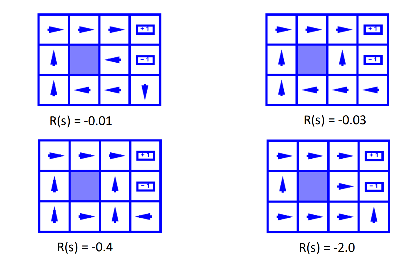
|
||||
|
||||
> [!NOTE]
|
||||
>
|
||||
> When $R(s)$ is small, the agent will prefer to take actions that avoids punishment in short term.
|
||||
|
||||
### The existence of the optimal policy
|
||||
|
||||
Theorem: for any Markov Decision Process
|
||||
|
||||
- There exists an optimal policy
|
||||
- There can be many optimal policies, but all optimal policies achieve the same optimal value function
|
||||
- There is always a deterministic optimal policy for any MDP
|
||||
|
||||
## Value Iteration
|
||||
|
||||
## Policy Iteration
|
||||
@@ -1,298 +0,0 @@
|
||||
# CSE510 Deep Reinforcement Learning (Lecture 4)
|
||||
|
||||
Markov Decision Process (MDP) Part II
|
||||
|
||||
## Recall from last lecture
|
||||
|
||||
An Finite MDP is defined by:
|
||||
|
||||
- A finite set of **states** $s \in S$
|
||||
- A finite set of **actions** $a \in A$
|
||||
- A **transition function** $T(s, a, s')$
|
||||
- Probability that a from s leads to $s'$, i.e.,
|
||||
$P(s'| s, a)$
|
||||
- Also called the model or the dynamics
|
||||
- A **reward function $R(s)$** ( Sometimes $R(s,a)$ or $R(s, a, s')$ )
|
||||
- A **start state**
|
||||
- Maybe a **terminal state**
|
||||
|
||||
A model for sequential decision making problem under uncertainty
|
||||
|
||||
### Optimal Policy and Bellman Optimality Equation
|
||||
|
||||
The goal for a MDP is to compute or learn an optimal policy.
|
||||
|
||||
- An **optimal policy** is one that achieves the highest value at any state
|
||||
|
||||
$$
|
||||
\pi^* = \arg\max_\pi V^\pi(s)
|
||||
$$
|
||||
|
||||
- We define the optimal value function using Bellman Optimality Equation
|
||||
|
||||
$$
|
||||
V^*(s) = R(s) + \gamma \max_{a\in A} \sum_{s'\in S} P(s'|s,a) V^*(s')
|
||||
$$
|
||||
|
||||
- The optimal policy is
|
||||
|
||||
$$
|
||||
\pi^*(s) = \arg\max_{a\in A} \sum_{s'\in S} P(s'|s,a) V^*(s')
|
||||
$$
|
||||
|
||||
### The Existence of the Optimal Policy
|
||||
|
||||
Theorem: for any Markov Decision Process
|
||||
|
||||
- There exists an optimal policy
|
||||
- There can be many optimal policies, but all optimal policies achieve the same optimal value function
|
||||
- There is always a deterministic optimal policy for any MDP
|
||||
|
||||
## Solve MDP
|
||||
|
||||
### Value Iteration
|
||||
|
||||
Repeatedly update an estimate of the optimal value function according to Bellman Optimality Equation.
|
||||
|
||||
1. Initialize an estimate for the value function arbitrarily
|
||||
|
||||
$$
|
||||
\hat{V}(s) \gets 0, \forall s \in S
|
||||
$$
|
||||
|
||||
2. Repeat, update:
|
||||
|
||||
$$
|
||||
\hat{V}(s) \gets R(s) + \gamma \max_{a\in A} \sum_{s'\in S} P(s'|s,a) \hat{V}(s'), \forall s \in S
|
||||
$$
|
||||
|
||||
<details>
|
||||
<summary>Example</summary>
|
||||
|
||||
Suppose we have a robot that can move in a 2D grid. with the following dynamics:
|
||||
|
||||
- with 80% probability, the robot moves in the direction of the action
|
||||
- with 10% probability, the robot moves in the direction of the action + 1 (wrap to left)
|
||||
- with 10% probability, the robot moves in the direction of the action - 1 (wrap to right)
|
||||
|
||||
The gird ($V^0(s)$) is:
|
||||
|
||||
|0|0|0|1|
|
||||
|0|*|0|-100|
|
||||
|0|0|0|0|
|
||||
|
||||
If we fun the value iteration with $\gamma = 0.9$, we can update the value function as follows:
|
||||
|
||||
$$
|
||||
V^1(s) = R(s) + \gamma \max_{a\in A} \sum_{s'\in S} P(s'|s,a) V^0(s')
|
||||
$$
|
||||
|
||||
On point $(3,3)$, the best action is to move to the goal state, so:
|
||||
|
||||
$$
|
||||
\begin{aligned}
|
||||
V^1((3,3)) &= R((3,3)) + \gamma \max_{a\in A} \sum_{s'\in S} P(s'|(3,3),\text{right}) V^0((3,4))
|
||||
&= 0+0.9 \times 0.8 \times 1 = 0.72
|
||||
\end{aligned}
|
||||
$$
|
||||
|
||||
On point $(3,4)$, the best action is to move up so that you can stay in the grid with $90\%$ probability, so:
|
||||
|
||||
$$
|
||||
\begin{aligned}
|
||||
V^1((3,4)) &= R((3,4)) + \gamma \max_{a\in A} \sum_{s'\in S} P(s'|(3,4),\text{up}) V^0((3,4))
|
||||
&= 1+0.9 \times (0.8+0.1) \times 1 = 1.81
|
||||
\end{aligned}
|
||||
$$
|
||||
|
||||
On $t=1$, the value on grid is:
|
||||
|
||||
|0|0|0.72|1.81|
|
||||
|0|*|0|-99.91|
|
||||
|0|0|0|0|
|
||||
|
||||
</details>
|
||||
|
||||
The general algorithm can be written as:
|
||||
|
||||
```python
|
||||
# suppose we defined the grid as previous example
|
||||
|
||||
grid = [
|
||||
[0, 0, 0, 1],
|
||||
[0, '*', 0, -100],
|
||||
[0, 0, 0, 0]
|
||||
]
|
||||
m,n = len(grid), len(grid[0])
|
||||
ACTIONS = {'up':(0,-1), 'down':(0,1), 'left':(-1,0), 'right':(1,0)}
|
||||
|
||||
gamma = 0.9
|
||||
V = value_iteration(gamma, ACTIONS, grid)
|
||||
print(V)
|
||||
|
||||
def get_reward(action, i, j):
|
||||
reward = 0
|
||||
reward += 0.8 * grid[i+action[0]][j+action[1]] if i+action[0] >= 0 and i+action[0] < m and j+action[1] >= 0 and j+action[1] < n and grid[i+action[0]][j+action[1]] != '*' else grid[i][j]
|
||||
reward += 0.1 * grid[i+action[0]][j+action[1]] if i+action[0] >= 0 and i+action[0] < m and j+action[1] >= 0 and j+action[1] < n and grid[i+action[0]][j+action[1]] != '*' else grid[i][j]
|
||||
reward += 0.1 * grid[i+action[0]][j+action[1]] if i+action[0] >= 0 and i+action[0] < m and j+action[1] >= 0 and j+action[1] < n and grid[i+action[0]][j+action[1]] != '*' else grid[i][j]
|
||||
return reward
|
||||
|
||||
def value_iteration(gamma, ACTIONS, V):
|
||||
V_new=[[0]*m for _ in range(n)]
|
||||
while True:
|
||||
for i in range(m):
|
||||
for j in range(n):
|
||||
s = (i, j)
|
||||
V_new[i][j] = V[i][j] + gamma * max(get_reward(action, i, j) for action.values() in ACTIONS)
|
||||
if max(abs(V_new[i][j] - V[i][j]) for i in range(m) for j in range(n)) < 1e-6:
|
||||
break
|
||||
V = V_new
|
||||
return V
|
||||
```
|
||||
|
||||
### Convergence of Value Iteration
|
||||
|
||||
Theorem: Value Iteration converges to the optimal value function $\hat{V}\to V^*$ as $t\to\infty$.
|
||||
|
||||
<details>
|
||||
<summary>Proof</summary>
|
||||
|
||||
For any estimate of the value function $\hat{V}$, we define the Bellman backup operator $\operatorname{B}:\mathbb{R}^{|S|}\to \mathbb{R}^{|S|}$ by
|
||||
|
||||
$$
|
||||
\operatorname{B}(\hat{V}(s)) = R(s) + \gamma \max_{a\in A} \sum_{s'\in S} P(s'|s,a) \hat{V}(s')
|
||||
$$
|
||||
|
||||
Note that $\operatorname{B}(V^*) = V^*$.
|
||||
|
||||
Since $\|\max_{x\in X}f(x)-\max_{x\in X}g(x)\|\leq \max_{x\in X}\|f(x)-g(x)\|$, for any value function $V_1$ and $V_2$, we have
|
||||
|
||||
$$
|
||||
\begin{aligned}
|
||||
|\operatorname{B}(V_1(s))-\operatorname{B}(V_2(s))|&= \gamma \left|\max_{a\in A} \sum_{s'\in S} P(s'|s,a) V_1(s')-\max_{a\in A} \sum_{s'\in S} P(s'|s,a) V_2(s')\right|\\
|
||||
&\leq \gamma \max_{a\in A} \left|\sum_{s'\in S} P(s'|s,a) V_1(s')-\sum_{s'\in S} P(s'|s,a) V_2(s')\right|\\
|
||||
&\leq \gamma \max_{a\in A} \sum_{s'\in S} P(s'|s,a) |V_1(s')-V_2(s')|\\
|
||||
&\leq \gamma \max_{s\in S}|V_1-V_2|
|
||||
\end{aligned}
|
||||
$$
|
||||
|
||||
</details>
|
||||
|
||||
Assume $0\leq \gamma < 1$, and reward $R(s)$ is bounded by $R_{\max}$.
|
||||
|
||||
Then
|
||||
|
||||
$$
|
||||
V^*(s)\leq \sum_{t=0}^\infty \gamma^t R_{\max} = \frac{R_{\max}}{1-\gamma}
|
||||
$$
|
||||
|
||||
Let $V^k$ be the value function after $k$ iterations of Value Iteration.
|
||||
|
||||
$$
|
||||
\max_{s\in S}|V^k(s)-V^*(s)|\leq \frac{R_{\max}}{1-\gamma}\gamma^k
|
||||
$$
|
||||
|
||||
#### Stopping condition
|
||||
|
||||
We can construct the optimal policy arbitrarily close to the optimal value function.
|
||||
|
||||
If $\|V^k-V^{k+1}\|<\epsilon$, then $\|V^k-V^*\|\leq \epsilon\frac{\gamma}{1-\gamma}$.
|
||||
|
||||
So we can select small $\epsilon$ to stop the iteration.
|
||||
|
||||
### Greedy Policy
|
||||
|
||||
Given a $V^k$ that is close to the optimal value $V^*$, the greedy policy is:
|
||||
|
||||
$$
|
||||
\pi_{g}(s) = \arg\max_{a\in A} \sum_{s'\in S} T(s',a,s') V^k(s')
|
||||
$$
|
||||
|
||||
Here $T(s',a,s')$ is the transition function between state $s'$ and $s$ with action $a$.
|
||||
|
||||
This selects the action looks best if we assume that we get value $V^k$ in one step.
|
||||
|
||||
#### Value of a greedy policy
|
||||
|
||||
If we define $V_g$ to be the value function of the greedy policy, then
|
||||
|
||||
This is not necessarily optimal, but it is a good approximation.
|
||||
|
||||
In homework, we will prove that if $\|V^k-V^*\|<\lambda$, then $\|V_g-V^*\|\leq 2\lambda\frac{\gamma}{1-\gamma}$.
|
||||
|
||||
So we can set stopping condition so that $V_g$ has desired accuracy to $V^*$.
|
||||
|
||||
There is a finite $\epsilon$ such that greedy policy is $\epsilon$-optimal.
|
||||
|
||||
### Problem of Value Iteration and Policy Iteration
|
||||
|
||||
- It is slow $O(|S|^2|A|)$
|
||||
- The max action at each state rarely changes
|
||||
- The policy converges before the value function
|
||||
|
||||
### Policy Iteration
|
||||
|
||||
Interleaving polity evaluation and policy improvement.
|
||||
|
||||
1. Initialize a random policy $\hat{\pi}$
|
||||
2. Compute the value function $V^{\pi}$
|
||||
3. Update the policy $\pi$ to be greedy policy with respect to $V^{\pi}$
|
||||
$$
|
||||
\pi(s)\gets \arg\max_{a\in A} \sum_{s'\in S} P(s'|s,a) V^{\pi}(s')
|
||||
$$
|
||||
4. Repeat until convergence
|
||||
|
||||
### Exact Policy Evaluation by Linear Solver
|
||||
|
||||
Let $V^{\pi}\in \mathbb{R}^{|S|}$ be a vector of values for each state, $r\in \mathbb{R}^{|S|}$ be a vector of rewards for each state.
|
||||
|
||||
Let $P^{\pi}\in \mathbb{R}^{|S|\times |S|}$ be a transition matrix for the policy $\pi$.
|
||||
|
||||
$$
|
||||
P^{\pi}_{ij} = P(s_{t+1}=i|s_t=j,a_t=\pi(s_t))
|
||||
$$
|
||||
|
||||
The Bellman equation for the policy can be written in vector form as:
|
||||
|
||||
$$
|
||||
\begin{aligned}
|
||||
V^{\pi} &= r + \gamma P^{\pi} V^{\pi} \\
|
||||
(I-\gamma P^{\pi})V^{\pi} &= r \\
|
||||
V^{\pi} &= (I-\gamma P^{\pi})^{-1} r
|
||||
\end{aligned}
|
||||
$$
|
||||
|
||||
- Proof involves showing that each iteration is also a contraction and monotonically improve the policy
|
||||
- Convergence to the exact optimal policy
|
||||
- The number of policies is finite
|
||||
|
||||
In real world, policy iteration is usually faster than value iteration.
|
||||
|
||||
#### Policy Iteration Complexity
|
||||
|
||||
- Each iteration runs in polynomial time in the number of states and actions
|
||||
- There are at most |A|n policies and PI never repeats a policy
|
||||
- So at most an exponential number of iterations
|
||||
- Not a very good complexity bound
|
||||
- Empirically O(n) iterations are required
|
||||
- Challenge: try to generate an MDP that requires more than that n iterations
|
||||
|
||||
### Generalized Policy Iteration
|
||||
|
||||
- Generalized Policy Iteration (GPI): any interleaving of policy evaluation and policy improvement
|
||||
- independent of their granularity and other details of the two processes
|
||||
|
||||
### Summary
|
||||
|
||||
#### Policy Iteration vs Value Iteration
|
||||
|
||||
- **PI has two loops**: inner loop (evaluate $V^{\pi}$)
|
||||
and outer loop (improve $\pi$)
|
||||
- **VI has one loop**: repeatedly apply
|
||||
$V^{k+1}(s) = \max_{a\in A} [r(s,a) + \gamma \sum_{s'\in S} P(s'|s,a) V^k(s')]$
|
||||
- **Trade-offs**:
|
||||
- PI converges in few outer steps if you can evaluate quickly/accurately;
|
||||
- VI avoids expensive exact evaluation, doing cheaper but many Bellman optimality updates.
|
||||
- **Modified Policy Iteration**: partial evaluation + improvement.
|
||||
|
||||
- **Modified Policy Iteration**: partial evaluation + improvement.
|
||||
@@ -1,242 +0,0 @@
|
||||
# CSE510 Deep Reinforcement Learning (Lecture 5)
|
||||
|
||||
## Passive Reinforcement Learning
|
||||
|
||||
New twist: don't know T or R
|
||||
|
||||
- i.e. we don't know which states are good or what the actions do
|
||||
- Must actually try actions and states out to learn
|
||||
|
||||
### Passive learning and active learning
|
||||
|
||||
Passive Learning
|
||||
|
||||
- The agent has a fixed policy and tries to learn the utilities of states by observing the world go by
|
||||
- Analogous to policy evaluation
|
||||
- Often serves as a component of active learning algorithms
|
||||
- Often inspires active learning algorithms
|
||||
|
||||
Active Learning
|
||||
|
||||
- The agent attempts to find an optimal (or at least good) policy by acting in the world
|
||||
- Analogous to solving the underlying MDP, but without first being given the MDP model
|
||||
|
||||
### Model-based vs. Model-free RL
|
||||
|
||||
Model-based RL
|
||||
|
||||
- Learn the MDP model, or an approximate of it
|
||||
- Use it for policy evaluation or to find the optimal policy
|
||||
|
||||
Example as human: learn to navigate by exploring the environment
|
||||
|
||||
Model-free RL
|
||||
|
||||
- Derive the optimal policy without explicitly learning the model
|
||||
- Useful when model is difficult to represent and/or learn
|
||||
|
||||
Example as human: learn to walk, talk based on reflection. (don't need to know law of physics).
|
||||
|
||||
### Small vs. Huge MDPs
|
||||
|
||||
We will first cover RL methods for small MDPs
|
||||
|
||||
- MDPs where the number of states and actions is reasonably small
|
||||
- These algorithms will inspire more advanced methods
|
||||
|
||||
Later we will cover algorithms for huge MDPs
|
||||
|
||||
- Function Approximation Methods
|
||||
- Policy Gradient Methods
|
||||
- Actor-Critic Methods
|
||||
|
||||
### Problem settings
|
||||
|
||||
Suppose given a stationary policy, want to determine how good it is.
|
||||
|
||||
We want to estimate $V^\pi(s)$, but not given:
|
||||
|
||||
- translation matrix
|
||||
- reward function
|
||||
|
||||
### Monte Carlo direct estimation (model-free)
|
||||
|
||||
Also called Direct Estimation.
|
||||
|
||||
```python
|
||||
def monte_carlo_direct_estimation(policy, env, num_episodes):
|
||||
V = {}
|
||||
for episode in range(num_episodes):
|
||||
state = env.reset()
|
||||
while not env.done:
|
||||
action = policy.act(state)
|
||||
next_state, reward, done = env.step(action)
|
||||
V[state] += reward
|
||||
state = next_state
|
||||
return {s: V[s] / num_episodes for s in V}
|
||||
```
|
||||
|
||||
Estimate $V^\pi(s)$ by average total reward of episodes containing state $s$.
|
||||
|
||||
**Reward to go** of state s is the sum of the (discounted) rewards from the state until a terminal state is reached.
|
||||
|
||||
Drawback:
|
||||
|
||||
- Need large number of episodes to get accurate estimate
|
||||
- Does not exploit Bellman constrains on policy values.
|
||||
|
||||
### Adaptive Dynamic Programming (ADP) (model-based)
|
||||
|
||||
- Follow the policy for a while
|
||||
- Estimate transition model based on obsercations
|
||||
- Learn reward function
|
||||
- Use estimated model to compute utilities of policy
|
||||
|
||||
$$
|
||||
V^\pi(s) = R(s) + \gamma \sum_{s'\in S} T(s,a,s') V^\pi(s')
|
||||
$$
|
||||
|
||||
```python
|
||||
def adaptive_dynamic_programming(policy, env, num_episodes, steps_per_episode):
|
||||
V = {}
|
||||
for episode in range(num_episodes):
|
||||
state = env.reset()
|
||||
while not env.done:
|
||||
action = policy.act(state, steps_per_episode)
|
||||
next_state, reward, done = env.step(action)
|
||||
V[state] += reward
|
||||
state = next_state
|
||||
return {s: V[s] / num_episodes for s in V}
|
||||
```
|
||||
|
||||
Drawback:
|
||||
|
||||
- Still need full DP policy evaluation after certain steps.
|
||||
|
||||
### Temporal difference learning (model-free)
|
||||
|
||||
- Do local updates of utility/value function on a **per-action** basis
|
||||
- Don't try to estimate the entire transition function
|
||||
- For each transition from $s$ to $s'$, update:
|
||||
$$
|
||||
V^\pi(s) \gets V^\pi(s) + \alpha (R(s) + \gamma V^\pi(s') - V^\pi(s))
|
||||
$$
|
||||
|
||||
Here $\alpha$ is the learning rate, $\gamma$ is the discount factor.
|
||||
|
||||
```python
|
||||
def temporal_difference_learning(policy, env, num_episodes):
|
||||
V = {}
|
||||
for episode in range(num_episodes):
|
||||
state = env.reset()
|
||||
while not env.done:
|
||||
action = policy.act(state)
|
||||
next_state, reward, done = env.step(action)
|
||||
V[state] += alpha * (reward + gamma * V[next_state] - V[state])
|
||||
state = next_state
|
||||
return V
|
||||
```
|
||||
|
||||
Drawback:
|
||||
|
||||
- requires more training experience (epochs) than ADP but much less computation per epoch
|
||||
- Choice depends on relative cost of experience vs. computation
|
||||
|
||||
#### Online Mean Estimation algorithm
|
||||
|
||||
Suppose we want to incrementally computer the mean of a stream of numbers.
|
||||
|
||||
$$
|
||||
(x_1, x_2, \ldots)
|
||||
$$
|
||||
|
||||
Given a new sample $x_{n+1}$, the new mean is the old estimate (for $n$ samples) plus the weighted difference between the new sample and the old estimate.
|
||||
|
||||
$$
|
||||
\begin{aligned}
|
||||
\hat{X}_{n+1} &= \frac{1}{n+1} \sum_{i=1}^{n+1} x_i \\
|
||||
&= \frac{1}{n}\sum_{i=1}^{n} x_i + \frac{1}{n+1} x_{n}-\frac{1}{n}\hat{X}_n\\
|
||||
&= \hat{x}_{n} +\frac{1}{n+1} \left[x_{n+1} +\sum_{i=1}^{n} x_i-\frac{n+1}{n}\sum_{i=1}^{n} x_i\right]\\
|
||||
&= \hat{x}_{n} + \frac{1}{n+1} (x_{n+1} - \hat{X}_n)
|
||||
\end{aligned}
|
||||
$$
|
||||
|
||||
### Summary of passive RL
|
||||
|
||||
**Monte-Carlo Direct Estimation (model-free)**
|
||||
|
||||
- Simple to implement
|
||||
- Each update is fast
|
||||
- Does not exploit Bellman constraints
|
||||
- Converges slowly
|
||||
|
||||
**Adaptive Dynamic Programming (model-based)**
|
||||
|
||||
- Harder to implement
|
||||
- Each update is a full policy evaluation (expensive)
|
||||
- Fully exploits Bellman constraints
|
||||
- Fast convergence (in terms of updates)
|
||||
|
||||
**Temporal Difference Learning (model-free)**
|
||||
|
||||
- Update speed and implementation similar to direct estimation
|
||||
- Partially exploits Bellman constraints---adjusts state to 'agree' with observed successor
|
||||
- Not all possible successors as in ADP
|
||||
- Convergence speed in between direct estimation and ADP
|
||||
|
||||
### Between ADP and TD
|
||||
|
||||
- Moving TD toward ADP
|
||||
- At each step perform TD updates based on observed transition and "imagined" transitions based on initial trajectory tests. (model-based)
|
||||
- Imagined transition are generated using estimated model
|
||||
- The more imagined transitions used, the more like ADP
|
||||
- Making estimate more consistent with next state distribution
|
||||
- Converges in the limit of infinite imagined transitions to ADP
|
||||
- Trade-off computational and experience efficiency
|
||||
- More imagined transitions require more time per step, but fewer steps of actual experience
|
||||
|
||||
## Active Reinforcement Learning
|
||||
|
||||
### Naive Model-Based Approach
|
||||
|
||||
1. Act Randomly for a (long) time
|
||||
- Or systematically explore all possible actions
|
||||
2. Learn
|
||||
- Transition function
|
||||
- Reward function
|
||||
3. Use value iteration, policy iteration, ...
|
||||
4. Follow resulting policy
|
||||
|
||||
This will work if step 1 is running long enough. And there is no dead-end for policy testing.
|
||||
|
||||
Drawback:
|
||||
|
||||
- Long time to converge
|
||||
|
||||
### Revision of Naive Approach
|
||||
|
||||
1. Start with an initial (uninformed) model
|
||||
2. Solve for the optimal policy given the current model (using value or policy iteration)
|
||||
3. Execute an action suggested by the policy in the current state
|
||||
4. Update the estimated model based on the observed transition
|
||||
5. Goto 2
|
||||
|
||||
This is just like ADP but we follow the greedy policy suggested by current value estimate.
|
||||
|
||||
**Will this work?**
|
||||
|
||||
No. Can get stuck in local minima.
|
||||
|
||||
#### Exploration vs. Exploitation
|
||||
|
||||
Two reasons to take an action in RL:
|
||||
|
||||
- **Exploitation**: To try to get reward. We exploit our current knowledge to get a payoff.
|
||||
- **Exploration**: Get more information about the world. How do we know if there is not a pot of gold around the corner?
|
||||
|
||||
- To explore we typically need to take actions that do not seem best according to our current model
|
||||
- Managing the trade-off between exploration and exploitation is a critical issue in RL
|
||||
- Basic intuition behind most approaches:
|
||||
- Explore more when knowledge is weak
|
||||
- Exploit more as we gain knowledge
|
||||
|
||||
@@ -1,247 +0,0 @@
|
||||
# CSE510 Deep Reinforcement Learning (Lecture 6)
|
||||
|
||||
## Active reinforcement learning
|
||||
|
||||
### Exploration vs. Exploitation
|
||||
|
||||
- **Exploitation**: To try to get reward. We exploit our current knowledge to get a payoff.
|
||||
- **Exploration**: Get more information about the world. How do we know if there is not a pot of gold around the corner?
|
||||
|
||||
- To explore we typically need to take actions that do not seem best according to our current model
|
||||
- Managing the trade-off between exploration and exploitation is a critical issue in RL
|
||||
- Basic intuition behind most approaches
|
||||
- Explore more when knowledge is weak
|
||||
- Exploit more as we gain knowledge
|
||||
|
||||
### ADP-based RL
|
||||
|
||||
Model based
|
||||
|
||||
1. Start with an initial (uninformed) model
|
||||
2. solve for optimal policy given the current model (using value or policy iteration)
|
||||
3. Take action according to an **exploration/exploitation** policy
|
||||
4. Update estimated model based on observed transition
|
||||
5. Goto 2
|
||||
|
||||
#### Exploration/Exploitation policy
|
||||
|
||||
**Greedy action** is the action maximizing estimated $Q$ value
|
||||
|
||||
$$
|
||||
Q(s,a) = R(s) + \gamma \max_{s'\in S} P(s,a,s')V(s')
|
||||
$$
|
||||
|
||||
- where $V$ is current optimal value function estimate (based on current model), and $R, T$ are current estimates of model
|
||||
- $Q(s,a)$ is the expected value of taking action $a$ in state $s$ and then getting estimated value $V(s')$ for the next state $s'$
|
||||
|
||||
Want an exploration policy that is **greedy in the limit of infinite exploration** (GLIE)
|
||||
|
||||
- Try each action in each state and unbounded number of times
|
||||
- Guarantees convergence
|
||||
|
||||
**GLIE**: Greedy in the limit of infinite exploration
|
||||
|
||||
#### Greedy Policy 1
|
||||
|
||||
On time step $t$ select random action with probability $p(t)$ and greedy action with probability $1-p(t)$
|
||||
|
||||
$p(t) = \frac{1}{t}$ will lead to convergence, but is slow.
|
||||
|
||||
> [!TIP]
|
||||
>
|
||||
> In practice, it's common to simply set $p(t) = \epsilon$ for all $t$.
|
||||
|
||||
#### Greedy Policy 2
|
||||
|
||||
Boltzmann exploration
|
||||
|
||||
Selection action with probability,
|
||||
|
||||
$$
|
||||
Pr(a\mid s)=\frac{\exp(Q(s,a)/T)}{\sum_{a'\in A}\exp(Q(s,a')/T)}
|
||||
$$
|
||||
|
||||
$T$ is the temperature. Large $T$ means that each action has about the same probability. Small $T$ leads to more greedy behavior.
|
||||
|
||||
Typically start with large $T$ and decrease with time.
|
||||
|
||||
<details>
|
||||
<summary>Example: impact of temperature</summary>
|
||||
|
||||
Suppose we have two actions and that $Q(s,a_1) = 1$ and $Q(s,a_2) = 0$.
|
||||
|
||||
When $T=10$, we have
|
||||
|
||||
$$
|
||||
Pr(a_1\mid s)=\frac{\exp(1/10)}{\exp(1/10)+\exp(2/10)}=0.48
|
||||
$$
|
||||
|
||||
$$
|
||||
Pr(a_2\mid s)=\frac{\exp(2/10)}{\exp(1/10)+\exp(2/10)}=0.52
|
||||
$$
|
||||
|
||||
When $T=1$, we have
|
||||
|
||||
$$
|
||||
Pr(a_1\mid s)=\frac{\exp(1/1)}{\exp(1/1)+\exp(2/1)}=0.27
|
||||
$$
|
||||
|
||||
$$
|
||||
Pr(a_2\mid s)=\frac{\exp(2/1)}{\exp(1/1)+\exp(2/1)}=0.73
|
||||
$$
|
||||
|
||||
When $T=0.1$, we have
|
||||
|
||||
$$
|
||||
Pr(a_1\mid s)=\frac{\exp(1/0.1)}{\exp(1/0.1)+\exp(2/0.1)}=0.02
|
||||
$$
|
||||
|
||||
$$
|
||||
Pr(a_2\mid s)=\frac{\exp(2/0.1)}{\exp(1/0.1)+\exp(2/0.1)}=0.98
|
||||
$$
|
||||
|
||||
</details>
|
||||
|
||||
### (Alternative Model-Based RL) Optimistic Exploration: Rmax [Brafman & Tennenholtz, 2002]
|
||||
|
||||
1. Start with an **optimistic model**
|
||||
- (assign largest possible reward to "unexplored states")
|
||||
- (actions from "unexplored states" only self transition)
|
||||
2. Solve for optimal policy in optimistic model (standard VI)
|
||||
3. Take greedy action according to the computed policy
|
||||
4. Update optimistic estimated model
|
||||
- (if a state becomes "known" then use its true statistics)
|
||||
5. Goto 2
|
||||
|
||||
Agent always acts greedily according to a model that assumes
|
||||
all "unexplored" states are maximally rewarding
|
||||
|
||||
#### Implementation for optimistic model
|
||||
|
||||
- Keep track of number of times a state-action pair is tried
|
||||
- If $N(s, a) < N_e$ then $T(s,a,s)=1$ and $R(s) = Rmax$ in optimistic model,
|
||||
- Otherwise, $T(s,a,s’)$ and $R(s)$ are based on estimates obtained from the $N_e$ experiences (the estimate of true model)
|
||||
- $N_e$ can be determined by using Chernoff Bound
|
||||
- An optimal policy for this optimistic model will try to reach unexplored states (those with unexplored actions) since it can stay at those states and accumulate maximum reward
|
||||
- Never explicitly explores. Is always greedy, but with respect to an optimistic outlook.
|
||||
|
||||
```pseudocode
|
||||
Algorithm: (for Infinite horizon RL problems)
|
||||
Initialize $\hat{p}, \hat{r}$, and $N(s,a)$ For $t = 1, 2, ...$
|
||||
1. Build an optimistic reward model $(Q(s,a))_{s,a}$ from $\hat{p}, \hat{r}$, and $N(s,a)$
|
||||
2. Select action $a(t)$ maximizing $Q(s(t),a)$ over $A_{s(t)}$
|
||||
3. Observe the transition to $s(t+1)$ and collect reward $r(s(t),a(t))$ according to $\hat{p}$
|
||||
4. Update $\hat{p}, \hat{r}$, and $N(s,a)$
|
||||
```
|
||||
|
||||
#### Efficiency of Rmax
|
||||
|
||||
If the model is very completely learned (i.e. $N(s, a) = N_e$ for all $s, a$), then Rmax will be near optimal.
|
||||
|
||||
Results how that this will happen "quickly" in terms of number of steps.
|
||||
|
||||
General proof strategy: **PAC Guarantee (Roughly speaking):** There is a value $N_e$, such that with high probability the Rmax algorithm will select at most a polynomial number of actions with value less than $\epsilon$ of optimal.
|
||||
|
||||
RL can be solved in poly-time in number of actions, number of states, and discount factor.
|
||||
|
||||
### TD-based Active RL
|
||||
|
||||
1. Start with initial value function
|
||||
2. Take action from an **exploration/exploitation** policygiving new state $s'$ (should converge to optimal policy)
|
||||
3. **Update** estimated model (To compute the exploration/exploitation policy.)
|
||||
4. Perform TD update
|
||||
$$
|
||||
V(s) \gets V(s) + \alpha (R(s) + \gamma V(s') - V(s))
|
||||
$$
|
||||
$V(s)$ is new estimate of optimal value function at state $s$.
|
||||
5. Goto 2
|
||||
|
||||
Given the usual assumptions about learning rate and GLIE, TD will converge to an optimal value function!
|
||||
|
||||
- Exploration/Exploitation policy requires computing $argmax Q(s, a)$ for the exploitation part of the policy
|
||||
- Computing $argmax Q(s, a)$ requires $T$ in addition to $V$
|
||||
- Thus TD-learning must still maintain an estimated model for action selection
|
||||
- It is computationally more efficient at each step compared to Rmax (i.e., optimistic exploration)
|
||||
- TD-update vs. Value Iteration
|
||||
- But model requires much more memory than value function
|
||||
- Can we get a model-fee variant?
|
||||
|
||||
### Q-learning
|
||||
|
||||
Instead of learning the optimal value function $V$, directly learn the optimal $Q$ function.
|
||||
|
||||
Recall $Q(s, a)$ is the expected value of taking action $a$ in state $s$ and then
|
||||
following the optimal policy thereafter
|
||||
|
||||
Given the $Q$ function we can act optimally by selecting action greedily according to $Q(s, a)$ without a model
|
||||
|
||||
The optimal $Q$-function satisfies $V(s) = \max_{a'\in A} Q(s, a')$ which gives:
|
||||
|
||||
$$
|
||||
\begin{aligned}
|
||||
Q(s,a) &= R(s) + \gamma \sum_{s'\in S} T(s,a,s') V(s')\\
|
||||
&= R(s) + \gamma \sum_{s'\in S} T(s,a,s') \max_{a'\in A} Q(s',a')\\
|
||||
\end{aligned}
|
||||
$$
|
||||
|
||||
How can we learn the $Q$-function directly?
|
||||
|
||||
#### Q-learning implementation
|
||||
|
||||
Model-free reinforcement learning
|
||||
|
||||
1. Start with initial Q-values (e.g. all zeros)
|
||||
2. Take action from an **exploration/exploitation** policy giving new state $s'$ (should converge to optimal policy)
|
||||
3. Perform TD update
|
||||
$$
|
||||
Q(s,a) \gets Q(s,a) + \alpha (R(s) + \gamma \max_{a'\in A} Q(s',a') - Q(s,a))
|
||||
$$
|
||||
$Q(s,a)$ is current estimate of optimal Q-value for state $s$ and action $a$.
|
||||
4. Goto 2
|
||||
|
||||
- Does not require model since we learn the Q-value function directly
|
||||
- Use explicit $|S|\times |A|$ table to store Q-values
|
||||
- Off-policy learning: the update does not depend on the actual next action
|
||||
- The exploration/exploitation policy directly uses $Q$-values
|
||||
|
||||
#### Convergence of Q-learning
|
||||
|
||||
Q-learning converges to the optimal Q-value in the limit with probability 1 if:
|
||||
|
||||
- Every state-action pair is visited infinitely often
|
||||
- Learning rate decays just so: $\sum_{t=1}^{\infty} \alpha(t) = \infty$ and $\sum_{t=1}^{\infty} \alpha(t)^2 < \infty$
|
||||
|
||||
#### Speedup for Goal-Based Problems
|
||||
|
||||
- **Goal-Based Problem**: receive big reward in goal state and then transition to terminal state
|
||||
- Initializing $Q(s, a)$ for all $s \in S$ and $a \in A$ to zeros and then observing the following sequence of (state, reward, action) triples
|
||||
- $(s0, 0, a0) (s1, 0, a1) (s2, 10, a2) (terminal,0)$
|
||||
- The sequence of Q-value updates would result in: $Q(s0, a0) = 0$, $Q(s1, a1) =0$, $Q(s2, a2)=10$
|
||||
- So nothing was learned at $s0$ and $s1$
|
||||
- Next time this trajectory is observed we will get non-zero for $Q(s1, a1)$ but still $Q(s0, a0)=0$
|
||||
|
||||
|
||||
From the example we see that it can take many learning trials for the final reward to "back propagate" to early state-action pairs
|
||||
|
||||
- Two approaches for addressing this problem:
|
||||
1. Trajectory replay: store each trajectory and do several iterations of Q-updates on each one
|
||||
2. Reverse updates: store trajectory and do Q-updates in reverse order
|
||||
- In our example (with learning rate and discount factor equal to 1 for ease of illustration) reverse updates would give
|
||||
- $Q(s2,a2) = 10$, $Q(s1,a1) = 10$, $Q(s0,a0)=10$
|
||||
|
||||
### Off-policy vs on-policy RL
|
||||
|
||||
### SARSA
|
||||
|
||||
1. Start with initial Q-values (e.g. all zeros)
|
||||
2. Take action $a_n$ on state $s_n$ from an $\epsilon$-greedy policy giving new state $s_{n+1}$
|
||||
3. Take action $a_{n+1}$ on state $s_{n+1}$ from an $\epsilon$-greedy
|
||||
4. Perform TD update
|
||||
$$
|
||||
Q(s_n,a_n) \gets Q(s_n,a_n) + \alpha (R(s_n) + \gamma Q(s_{n+1},a_{n+1}) - Q(s_n,a_n))
|
||||
$$
|
||||
5. Goto 2
|
||||
|
||||
> [!NOTE]
|
||||
>
|
||||
> Compared with Q-learning, SARSA (on-policy) usually takes more "safer" actions.
|
||||
@@ -1,190 +0,0 @@
|
||||
# CSE510 Deep Reinforcement Learning (Lecture 7)
|
||||
|
||||
## Large Scale RL
|
||||
|
||||
So far we have represented value functions by a lookup table
|
||||
|
||||
- Every state s has an entry V(s), or
|
||||
- Every state-action pair (s, a) has an entry Q(s, a)
|
||||
|
||||
Reinforcement learning should be used to solve large problems, e.g.
|
||||
|
||||
- Backgammon: 10^20 states
|
||||
- Computer Go: 10^170 states
|
||||
- Helicopter, robot, ...: enormous continuous state space
|
||||
|
||||
Tabular methods clearly cannot handle this.. why?
|
||||
|
||||
- There are too many states and/or actions to store in memory
|
||||
- It is too slow to learn the value of each state individually
|
||||
- You cannot generalize across states!
|
||||
|
||||
### Value Function Approximation (VFA)
|
||||
|
||||
Solution for large MDPs:
|
||||
|
||||
- Estimate the value function using a function approximator
|
||||
|
||||
**Value function approximation (VFA)** replaces the table with general parameterize form:
|
||||
|
||||
$$
|
||||
\hat{V}(s, \theta) \approx V_\pi(s)
|
||||
$$
|
||||
|
||||
or
|
||||
|
||||
$$
|
||||
\hat{Q}(s, a, \theta) \approx Q_\pi(s, a)
|
||||
$$
|
||||
|
||||
Benefit:
|
||||
|
||||
- Can generalize across states
|
||||
- Save memory (only need to store the function approximator parameters)
|
||||
|
||||
### End-to-End RL
|
||||
|
||||
End-to-end RL methods replace the hand-designed state representation with raw observations.
|
||||
|
||||
- Good: We get rid of manual design of state representations
|
||||
- Bad: we need tons of data to train the network since O_t usually WAY more high dimensional than hand-designed S_t
|
||||
|
||||
## Function Approximation
|
||||
|
||||
- Linear function approximation
|
||||
- Neural network function approximation
|
||||
- Decision tree function approximation
|
||||
- Nearest neighbor
|
||||
- ...
|
||||
|
||||
In this course, we will focus on **Linear combination of features** and **Neural networks**.
|
||||
|
||||
Today we will do Deep neural networks (fully connected and convolutional).
|
||||
|
||||
### Artificial Neural Networks
|
||||
|
||||
#### Neuron
|
||||
|
||||
$f(x) = \mathbb{R}^k\to \mathbb{R}$
|
||||
|
||||
$z=a_1w_1+a_2w_2+\cdots+a_kw_k+b$
|
||||
|
||||
$a_1,a_2,\cdots,a_k$ are the inputs, $w_1,w_2,\cdots,w_k$ are the weights, $b$ is the bias.
|
||||
|
||||
Then we have activation function $\sigma(z)$ (usually non-linear)
|
||||
|
||||
##### Activation functions
|
||||
|
||||
ReLU (rectified linear unit):
|
||||
|
||||
$$
|
||||
\text{ReLU}(x) = \max(0, x)
|
||||
$$
|
||||
|
||||
- Bounded below by 0.
|
||||
- Non-vanishing gradient.
|
||||
- No upper bound.
|
||||
|
||||
Sigmoid:
|
||||
|
||||
$$
|
||||
\text{Sigmoid}(x) = \frac{1}{1 + e^{-x}}
|
||||
$$
|
||||
|
||||
- Always positive.
|
||||
- Bounded between 0 and 1.
|
||||
- Strictly increasing.
|
||||
|
||||
> [!TIP]
|
||||
>
|
||||
> Use relu for previous layers, use sigmoid for output layer.
|
||||
>
|
||||
> For fully connected shallow networks, you may use more sigmoid layers.
|
||||
|
||||
We can use parallel computing techniques to speed up the computation.
|
||||
|
||||
#### Universal Approximation Theorem
|
||||
|
||||
Any continuous function can be approximated by a neural network with a single hidden layer.
|
||||
|
||||
(flat layer)
|
||||
|
||||
#### Why use deep neural networks?
|
||||
|
||||
Motivation from Biology
|
||||
|
||||
- Visual Cortex
|
||||
|
||||
Motivation from circuit theory
|
||||
|
||||
- Compact representation
|
||||
|
||||
Modularity
|
||||
|
||||
- More efficiently using data
|
||||
|
||||
In Practice: works better for many domains
|
||||
|
||||
- Hard to argue with results.
|
||||
|
||||
### Training Neural Networks
|
||||
|
||||
- Loss function
|
||||
- Model
|
||||
- Optimization
|
||||
|
||||
Empirical loss minimization framework:
|
||||
|
||||
$$
|
||||
\argmin_{\theta} \frac{1}{n} \sum_{i=1}^n \ell(f(x_i; \theta), y_i)+\lambda \Omega(\theta)
|
||||
$$
|
||||
|
||||
$\ell$ is the loss function, $f$ is the model, $\theta$ is the parameters, $\Omega$ is the regularization term, $\lambda$ is the regularization parameter.
|
||||
|
||||
Learning is cast as optimization.
|
||||
|
||||
- For classification problems, we would like to minimize classification error, e.g., logistic or cross entropy loss.
|
||||
- For regression problems, we would like to minimize regression error, e.g. L1 or L2 distance from groundtruth.
|
||||
|
||||
#### Stochastic Gradient Descent
|
||||
|
||||
Perform updates after seeing each example:
|
||||
|
||||
- Initialize: $\theta\equiv\{W^{(1)},b^{(1)},\cdots,W^{(L)},b^{(L)}\}$
|
||||
- For $t=1,2,\cdots,T$:
|
||||
- For each training example $(x^{(t)},y^{(t)})$:
|
||||
- Compute gradient: $\Delta = -\nabla_\theta \ell(f(x^{(t)}; \theta), y^{(t)})-\lambda\nabla_\theta \Omega(\theta)$
|
||||
- $\theta \gets \theta + \alpha \Delta$
|
||||
|
||||
Training a neural network, we need:
|
||||
|
||||
- Loss function
|
||||
- Procedure to compute the gradient
|
||||
- Regularization term
|
||||
|
||||
#### Mini-batch and Momentum
|
||||
|
||||
Make updates based on a mini-batch of examples (instead of a single example)
|
||||
|
||||
- the gradient is computed on the average regularized loss for that mini-batch
|
||||
- can give a more accurate estimate of the gradient
|
||||
|
||||
Momentum can use an exponential average of previous gradients.
|
||||
|
||||
$$
|
||||
\overline{\nabla}_\theta^{(t)}=\nabla_\theta \ell(f(x^{(t)}; \theta), y^{(t)})+\beta\overline{\nabla}_\theta^{(t-1)}
|
||||
$$
|
||||
|
||||
can get pass plateaus more quickly, by "gaining momentum".
|
||||
|
||||
### Convolutional Neural Networks
|
||||
|
||||
Overview of history:
|
||||
|
||||
- CNN
|
||||
- MLP
|
||||
- RNN/LSTM/GRU(Gated Recurrent Unit)
|
||||
- Transformer
|
||||
|
||||
|
||||
|
||||
@@ -1,78 +0,0 @@
|
||||
# CSE510 Deep Reinforcement Learning (Lecture 8)
|
||||
|
||||
## Convolutional Neural Networks
|
||||
|
||||
Another note in computer vision can be found here: [CSE559A Lecture 10](../CSE559A/CSE559A_L10#convolutional-layer)
|
||||
|
||||
Basically, it is a stack of different layers:
|
||||
|
||||
- Convolutional layer
|
||||
- Non-linearity layer
|
||||
- Pooling layer (or downsampling layer)
|
||||
- Fully connected layer
|
||||
|
||||
### Convolutional layer
|
||||
|
||||
Filtering: The math behind the matching.
|
||||
|
||||
1. Line up the feature and the image patch.
|
||||
2. Multiply each image pixel by the corresponding feature pixel.
|
||||
3. Add them up.
|
||||
4. Divide by the total number of pixels in the feature.
|
||||
|
||||
Idea of a convolutional neural network, in some sense, is to let the network "learn" the right filters for a specific task.
|
||||
|
||||
### Non-linearity Layer
|
||||
|
||||
> [!TIP]
|
||||
>
|
||||
> This is irrelevant to the lecture, but consider the following term:
|
||||
>
|
||||
> "Bounded rationality"
|
||||
|
||||
- Convolution is a linear operation
|
||||
- Non-linearity layer creates an activation map from the feature map generated by the convolutional layer
|
||||
- Consisting an activation function (an element-wise operation)
|
||||
- Rectified linear units (ReLUs) is advantageous over the traditional sigmoid or tanh activation functions
|
||||
|
||||
### Pooling layer
|
||||
|
||||
Shrinking the Image Stack
|
||||
|
||||
- Motivation: the activation maps can be large
|
||||
- Reducing the spacial size of the activation maps
|
||||
- Often after multiple stages of other layers (i.e., convolutional and non-linear layers)
|
||||
- Steps:
|
||||
1. Pick a window size (usually 2 or 3).
|
||||
2. Pick a stride (usually 2).
|
||||
3. Walk your window across your filtered images.
|
||||
4. From each window, take the maximum value.
|
||||
|
||||
Pros:
|
||||
|
||||
- Reducing the computational requirements
|
||||
- Minimizing the likelihood of overfitting
|
||||
|
||||
Cons:
|
||||
|
||||
- Aggressive reduction can limit the depth of a network and ultimately limit the performance
|
||||
|
||||
### Fully connected layer
|
||||
|
||||
- Multilayer perceptron (MLP)
|
||||
- Mapping the activation volume from previous layers into a class probability distribution
|
||||
- Non-linearity is built in the neurons, instead of a separate layer
|
||||
- Viewed as 1x1 convolution kernels
|
||||
|
||||
For classification: Output layer is a regular, fully connected layer with softmax non-linearity
|
||||
|
||||
- Output provides an estimate of the conditional probability of each class
|
||||
|
||||
> [!TIP]
|
||||
>
|
||||
> The golden triangle of machine learning:
|
||||
>
|
||||
> - Data
|
||||
> - Algorithm
|
||||
> - Computation
|
||||
|
||||
@@ -1,271 +0,0 @@
|
||||
# CSE510 Deep Reinforcement Learning (Lecture 9)
|
||||
|
||||
## Large state spaces
|
||||
|
||||
RL algorithms presented so far have little chance to solve real-world problems when the state (or action) space is large.
|
||||
|
||||
- not longer represent the $V$ or $Q$ function as explicit tables
|
||||
|
||||
Even if we had enough memory
|
||||
|
||||
- Never enough training data
|
||||
- Learning takes too long
|
||||
|
||||
What about large state spaces?
|
||||
|
||||
We will now study three other approaches
|
||||
|
||||
- Value function approximation
|
||||
- Policy gradient methods
|
||||
- Actor-critic methods
|
||||
|
||||
## RL with Function Approximation
|
||||
|
||||
Solution for large MDPs:
|
||||
|
||||
- Estimate value function using a function approximator
|
||||
|
||||
**Value function approximation (VFA)** replaces the table with general parameterize form:
|
||||
|
||||
$$
|
||||
\hat{V}(s, \theta) \approx V_\pi(s)
|
||||
$$
|
||||
|
||||
or
|
||||
|
||||
$$
|
||||
\hat{Q}(s, a, \theta) \approx Q_\pi(s, a)
|
||||
$$
|
||||
|
||||
Benefit:
|
||||
|
||||
- Generalization: those functions can be trained to map similar states to similar values
|
||||
- Reduce memory usage
|
||||
- Reduce computation time
|
||||
- Reduce experience needed to learn the V/Q
|
||||
|
||||
## Linear Function Approximation
|
||||
|
||||
Defined a set of state features $f_1(s),\ldots,f_n(s)$
|
||||
|
||||
- The features are used as our representation of the state
|
||||
- States with similar features values will be considered similar
|
||||
|
||||
A common approximation is to represent $V(s)$ as a linear combination of the features:
|
||||
|
||||
$$
|
||||
\hat{V}(s, \theta) = \theta_0 + \sum_{i=1}^n \theta_i f_i(s)
|
||||
$$
|
||||
|
||||
The approximation accuracy is fundamentally limited by the information provided by the features
|
||||
|
||||
Can we always defined features that allow for a perfect linear approximation?
|
||||
|
||||
- Yes. Assign each state an indicator feature. ($i$th feature is $1$ if and only if the $i$th state is present and $\theta_i$ represents value of $i$th state)
|
||||
- However, this requires a feature for each state, which is impractical for large state spaces. (no generalization)
|
||||
|
||||
<details>
|
||||
<summary>Example</summary>
|
||||
|
||||
Grid with no obstacles, deterministic actions U/D/L/R, no discounting, -1 reward everywhere except +10 at goal.
|
||||
|
||||
The grid is:
|
||||
|
||||
|4|5|6|7|8|9|10|
|
||||
|---|---|---|---|---|---|---|
|
||||
|3|4|5|6|7|8|9|
|
||||
|2|3|4|5|6|7|8|
|
||||
|1|2|3|4|5|6|7|
|
||||
|0|1|2|3|4|5|6|
|
||||
|0|0|1|2|3|4|5|
|
||||
|0|0|0|1|2|3|4|
|
||||
|
||||
Features for state $s=(x, y): f_1(s)=x, f_2(s)=y$ (just 2 features)
|
||||
|
||||
$$
|
||||
V(s) = \theta_0 + \theta_1 x + \theta_2 y
|
||||
$$
|
||||
|
||||
Is there a good linear approximation?
|
||||
|
||||
- Yes.
|
||||
- $\theta_0 =10, \theta_1 = -1, \theta_2 = -1$
|
||||
- (note upper right is origin)
|
||||
|
||||
$$
|
||||
V(s) = 10 - x - y
|
||||
$$
|
||||
|
||||
subtracts Manhattan dist from goal reward
|
||||
|
||||
---
|
||||
|
||||
However, for different grid, $V(s)=\theta_0 + \theta_1 x + \theta_2 y$ is not a good approximation.
|
||||
|
||||
|4|5|6|7|6|5|4|
|
||||
|---|---|---|---|---|---|---|
|
||||
|5|6|7|8|7|6|5|
|
||||
|6|7|8|9|8|7|6|
|
||||
|7|8|9|10|9|8|7|
|
||||
|6|7|8|9|8|7|6|
|
||||
|5|6|7|8|7|6|5|
|
||||
|4|5|6|7|6|5|4|
|
||||
|
||||
But we can include a new feature $z=|3-x|+|3-y|$ to get a good approximation.
|
||||
|
||||
$V(s) = \theta_0 + \theta_1 x + \theta_2 y + \theta_3 z$
|
||||
|
||||
> Usually, we need to define different approximation for different problems.
|
||||
|
||||
</details>
|
||||
|
||||
### Learning with Linear Function Approximation
|
||||
|
||||
Define a set of features $f_1(s),\ldots,f_n(s)$
|
||||
|
||||
- The features are used as our representation of the state
|
||||
- States with similar features values will be treated similarly
|
||||
- More complex functions require more features
|
||||
|
||||
$$
|
||||
\hat{V}(s, \theta) =\theta_0 + \sum_{i=1}^n \theta_i f_i(s)
|
||||
$$
|
||||
|
||||
Our goal is to learn good parameter values that approximate the value function well
|
||||
|
||||
- How can we do this?
|
||||
- Use TD-based RL and somehow update parameters based on each experience
|
||||
|
||||
#### TD-based learning with function approximators
|
||||
|
||||
1. Start with initial parameter values
|
||||
2. Take action according to an exploration/exploitation policy
|
||||
3. Update estimated model
|
||||
4. Perform TD update for each parameter
|
||||
$$
|
||||
\theta_i \gets \theta_i + \alpha \left(R(s_j)+\gamma \hat{V}_\theta(s_{j+1})- \hat{V}_\theta(s_j)\right)f_i(s_j)
|
||||
$$
|
||||
5. Goto 2
|
||||
|
||||
**The TD update for each parameter is**:
|
||||
|
||||
$$
|
||||
\theta_i \gets \theta_i + \alpha \left(v(s_j)-\hat{V}_\theta(s_j)\right)f_i(s_j)
|
||||
$$
|
||||
|
||||
<details>
|
||||
<summary>Proof from Gradient Descent</summary>
|
||||
|
||||
Our goal is to minimize the squared errors between our estimated value function at each target value:
|
||||
|
||||
$$
|
||||
E_j(\theta) = \frac{1}{2} \sum_{i=1}^n \left(\hat{V}_\theta(s_j)-v(s_j)\right)^2
|
||||
$$
|
||||
|
||||
Here $E_j(\theta)$ is the squared error of example $j$.
|
||||
|
||||
$\hat{V}_\theta(s_j)$ is our estimated value function at state $s_j$.
|
||||
|
||||
$v(s_j)$ is the true target value at state $s_j$.
|
||||
|
||||
After seeing $j$'th state, the **gradient descent rule** tells us that we can decrease error with respect to $E_j(\theta)$ by
|
||||
|
||||
$$
|
||||
\theta_i \gets \theta_i - \alpha \frac{\partial E_j(\theta)}{\partial \theta_i}
|
||||
$$
|
||||
|
||||
here $\alpha$ is the learning rate.
|
||||
|
||||
By the chain rule, we have:
|
||||
|
||||
$$
|
||||
\begin{aligned}
|
||||
\theta_i &\gets \theta_i -\alpha \frac{\partial E_j(\theta)}{\partial \theta_i} \\
|
||||
\theta_i -\alpha \frac{\partial E_j(\theta)}{\partial \theta_i} &=\theta_i - \alpha \frac{\partial E_j}{\partial \hat{V}_\theta(s_j)}\frac{\partial \hat{V}_\theta(s_j)}{\partial \theta_i}\\
|
||||
&= \theta_i - \alpha \left(\hat{V}_\theta(s_j)-v(s_j)\right)f_i(s_j)
|
||||
\end{aligned}
|
||||
$$
|
||||
|
||||
Note that $\frac{\partial E_j}{\partial \hat{V}_\theta(s_j)}=\hat{V}_\theta(s_j)-v(s_j)$
|
||||
|
||||
and $\frac{\partial \hat{V}_\theta(s_j)}{\partial \theta_i}=f_i(s_j)$
|
||||
|
||||
For the linear approximation function
|
||||
|
||||
$$
|
||||
\hat{V}_\theta(s_j) = \theta_0 + \sum_{i=1}^n \theta_i f_i(s_j)
|
||||
$$
|
||||
|
||||
we have $\frac{\partial \hat{V}_\theta(s_j)}{\partial \theta_i}=f_i(s_j)$
|
||||
|
||||
Thus the TD update for each parameter is:
|
||||
|
||||
$$
|
||||
\theta_i \gets \theta_i + \alpha \left(v(s_j)-\hat{V}_\theta(s_j)\right)f_i(s_j)
|
||||
$$
|
||||
|
||||
For linear functions, this update is guaranteed to converge to the best approximation for a suitable learning rate.
|
||||
|
||||
</details>
|
||||
|
||||
What we use for **target value** $v(s_j)$?
|
||||
|
||||
Use the TD prediction based on the next state $s_{j+1}$: (bootstrap learning)
|
||||
|
||||
$v(s)=R(s)+\gamma \hat{V}_\theta(s')$
|
||||
|
||||
So the TD update for each parameter is:
|
||||
|
||||
$$
|
||||
\theta_i \gets \theta_i + \alpha \left(R(s_j)+\gamma \hat{V}_\theta(s_{j+1})- \hat{V}_\theta(s_j)\right)f_i(s_j)
|
||||
$$
|
||||
|
||||
> [!NOTE]
|
||||
>
|
||||
> Initially, the value function may be full of zeros. It's better to use other dense reward to initialize the value function.
|
||||
|
||||
#### Q-function approximation
|
||||
|
||||
Instead of $f(s)$, we use $f(s,a)$ to approximate $Q(s,a)$:
|
||||
|
||||
State-action paris with similar feature values will be treated similarly.
|
||||
|
||||
More complex functions require more complex features.
|
||||
|
||||
$$
|
||||
\hat{Q}(s,a, \theta) = \theta_0 + \sum_{i=1}^n \theta_i f_i(s,a)
|
||||
$$
|
||||
|
||||
_Features are a function of state and action._
|
||||
|
||||
Just as fore TD, we can generalize Q-learning to updated parameters of the Q-function approximation
|
||||
|
||||
Q-learning with Linear Approximators:
|
||||
|
||||
1. Start with initial parameter values
|
||||
2. Take action according to an exploration/exploitation policy transition from $s$ to $s'$
|
||||
3. Perform TD update for each parameter
|
||||
$$
|
||||
\theta_i \gets \theta_i + \alpha \left(R(s)+\gamma \max_{a'\in A} \hat{Q}_\theta(s',a')- \hat{Q}_\theta(s,a)\right)f_i(s,a)
|
||||
$$
|
||||
4. Goto 2
|
||||
|
||||
> [!WARNING]
|
||||
>
|
||||
> Typically the space has many local minima and we no longer guarantee convergence.
|
||||
> However, it often works in practice.
|
||||
|
||||
Here $R(s)+\gamma \max_{a'\in A} \hat{Q}_\theta(s',a')$ is the estimate of $Q(s,a)$ based on an observed transition.
|
||||
|
||||
Note here $f_i(s,a)=\frac{\partial \hat{Q}_\theta(s,a)}{\partial \theta_i}$ This need to be computed in closed form.
|
||||
|
||||
## Deep Q-network (DQN)
|
||||
|
||||
This is a non-linear function approximator. That use deep neural networks to approximate the value function.
|
||||
|
||||
Goal is to seeking a single agent which can solve any human-level control problem.
|
||||
|
||||
- RL defined the objective (Q-value function)
|
||||
- DL learns the hierarchical feature representation
|
||||
|
||||
Use deep network to represent the value function:
|
||||
@@ -1,61 +0,0 @@
|
||||
export default {
|
||||
menu: {
|
||||
title: 'Home',
|
||||
type: 'menu',
|
||||
items: {
|
||||
index: {
|
||||
title: 'Home',
|
||||
href: '/'
|
||||
},
|
||||
about: {
|
||||
title: 'About',
|
||||
href: '/about'
|
||||
},
|
||||
contact: {
|
||||
title: 'Contact Me',
|
||||
href: '/contact'
|
||||
}
|
||||
},
|
||||
},
|
||||
Math3200'CSE510_link\s*:\s*(\{\s+.+\s+.+)\s+.+\s+.+\s+.+\s+(\},)'
|
||||
Math429'CSE510_link\s*:\s*(\{\s+.+\s+.+)\s+.+\s+.+\s+.+\s+(\},)'
|
||||
Math4111'CSE510_link\s*:\s*(\{\s+.+\s+.+)\s+.+\s+.+\s+.+\s+(\},)'
|
||||
Math4121'CSE510_link\s*:\s*(\{\s+.+\s+.+)\s+.+\s+.+\s+.+\s+(\},)'
|
||||
Math4201'CSE510_link\s*:\s*(\{\s+.+\s+.+)\s+.+\s+.+\s+.+\s+(\},)'
|
||||
Math416'CSE510_link\s*:\s*(\{\s+.+\s+.+)\s+.+\s+.+\s+.+\s+(\},)'
|
||||
Math401'CSE510_link\s*:\s*(\{\s+.+\s+.+)\s+.+\s+.+\s+.+\s+(\},)'
|
||||
CSE332S'CSE510_link\s*:\s*(\{\s+.+\s+.+)\s+.+\s+.+\s+.+\s+(\},)'
|
||||
CSE347'CSE510_link\s*:\s*(\{\s+.+\s+.+)\s+.+\s+.+\s+.+\s+(\},)'
|
||||
CSE442T'CSE510_link\s*:\s*(\{\s+.+\s+.+)\s+.+\s+.+\s+.+\s+(\},)'
|
||||
CSE5313'CSE510_link\s*:\s*(\{\s+.+\s+.+)\s+.+\s+.+\s+.+\s+(\},)'
|
||||
CSE510'CSE510_link\s*:\s*(\{\s+.+\s+.+)\s+.+\s+.+\s+.+\s+(\},)'
|
||||
CSE559A'CSE510_link\s*:\s*(\{\s+.+\s+.+)\s+.+\s+.+\s+.+\s+(\},)'
|
||||
CSE5519'CSE510_link\s*:\s*(\{\s+.+\s+.+)\s+.+\s+.+\s+.+\s+(\},)'
|
||||
Swap: {
|
||||
display: 'hidden',
|
||||
theme:{
|
||||
timestamp: true,
|
||||
}
|
||||
},
|
||||
index: {
|
||||
display: 'hidden',
|
||||
theme:{
|
||||
sidebar: false,
|
||||
timestamp: true,
|
||||
}
|
||||
},
|
||||
about: {
|
||||
display: 'hidden',
|
||||
theme:{
|
||||
sidebar: false,
|
||||
timestamp: true,
|
||||
}
|
||||
},
|
||||
contact: {
|
||||
display: 'hidden',
|
||||
theme:{
|
||||
sidebar: false,
|
||||
timestamp: true,
|
||||
}
|
||||
}
|
||||
}
|
||||
@@ -1,112 +0,0 @@
|
||||
# CSE510 Deep Reinforcement Learning
|
||||
|
||||
CSE 5100
|
||||
|
||||
**Class meeting times and Locations:** Tue/Thur from 10-11:20 am (412A-01 ) in EADS Room 216
|
||||
|
||||
**Fall 2025**
|
||||
|
||||
## Instructor Information
|
||||
|
||||
**Chongjie Zhang**
|
||||
Office: McKelvey Hall 2010D
|
||||
Email: chongjie@wustl.edu
|
||||
|
||||
### Instructor's Office Hours:
|
||||
|
||||
Chongjie Zhang's Office Hours: Wednesdays 11:00 -12:00 am in Mckelvey Hall 2010D Or you may email me to make an appointment.
|
||||
|
||||
### TAs:
|
||||
|
||||
- Jianing Ye: jianing.y@wustl.edu
|
||||
- Kefei Duan: d.kefei@wustl.edu
|
||||
- Xiu Yuan: xiu@wustl.edu
|
||||
|
||||
**Office Hours:** Thursday 4:00pm -5:00pm in Mckelvey Hall 1030 (tentative) Or you may email TAs to make an appointment.
|
||||
|
||||
## Course Description
|
||||
|
||||
Deep Reinforcement Learning (RL) is a cutting-edge field at the intersection of artificial intelligence and decision-making. This course provides an in-depth exploration of the fundamental principles, algorithms, and applications of deep reinforcement learning. We start from the Markov Decision Process (MDP) framework and cover basic RL algorithms—value-based, policy-based, actor–critic, and model-based methods—then move to advanced topics including offline RL and multi-agent RL. By combining deep learning with reinforcement learning, students will gain the skills to build intelligent systems that learn from experience and make near-optimal decisions in complex environments.
|
||||
|
||||
The course caters to graduate and advanced undergraduate students. Student performance evaluation will revolve around written and programming assignments and the course project.
|
||||
|
||||
By the end of this course, students should be able to:
|
||||
|
||||
- Formalize sequential decision problems with MDPs and derive Bellman equations.
|
||||
- Understand and analyze core RL algorithms (DP, MC, TD).
|
||||
- Build, train, and debug deep value-based methods (e.g., DQN and key extensions).
|
||||
- Implement and compare policy-gradient and actor–critic algorithms.
|
||||
- Explain and apply exploration strategies and stabilization techniques in deep RL.
|
||||
- Grasp model-based RL pipelines.
|
||||
- Explain assumptions, risks, and evaluation pitfalls in offline RL; implement a baseline offline RL method.
|
||||
- Formulate multi-agent RL problems; implement and evaluate a CTDE or value-decomposition method.
|
||||
- Execute an end-to-end DRL project: problem selection, environment design, algorithm selection, experimental protocol, ablations, and reproducibility.
|
||||
|
||||
## Prerequisites
|
||||
|
||||
If you are unsure about any of these, please speak to the instructor.
|
||||
|
||||
- Proficiency in Python programming.
|
||||
- Programming experience with deep learning.
|
||||
- Research Experience (Not required, but highly recommended)
|
||||
- Mathematics: Linear Algebra (MA 429 or MA 439 or ESE 318), Calculus III (MA 233), Probability & Statistics.
|
||||
|
||||
One of the following:
|
||||
- a) CSE 412A: Intro to A.I., or
|
||||
- b) a Machine Learning course (CSE 417T or ESE 417).
|
||||
|
||||
## Textbook
|
||||
|
||||
**Primary text** (optional but recommended): Sutton & Barto, Reinforcement Learning: An Introduction (2nd ed., online). We will not cover all of the chapters and, from time to time, cover topics not contained in the book.
|
||||
|
||||
**Additional references:** Russell & Norvig, Artificial Intelligence: A Modern Approach (4th ed.); OpenAI Spinning Up in Deep RL tutorial.
|
||||
|
||||
## Homeworks
|
||||
|
||||
There will be a total of three homework assignments distributed throughout the semester. Each assignment will be accessible on Canvas, allowing you approximately two weeks to finish and submit it before the designated deadline.
|
||||
|
||||
Late work will not be accepted. If you have a documented medical or emergency reason, contact the TAs as soon as possible.
|
||||
|
||||
**Collaboration:** Discussion of ideas is encouraged, but your write‑up and code must be your own. Acknowledge any collaborators and external resources.
|
||||
|
||||
**Academic Integrity:** Do not copy from peers or online sources. Violations will be referred per university policy.
|
||||
|
||||
## Final Project
|
||||
|
||||
A research‑level project of your choice that demonstrates mastery of DRL concepts and empirical methodology. Possible directions include: (a) improving an existing approach, (b) tackling an unsolved task/benchmark, (c) reproducing and extending a recent paper, or (d) creating a new task/problem relevant to RL.
|
||||
|
||||
**Team size:** 1–2 students by default (contact instructor/TAs for approval if proposing a larger team).
|
||||
|
||||
### Milestones:
|
||||
|
||||
- **Proposal:** ≤ 2 pages outlining problem, related work, methodology, evaluation plan, and risks.
|
||||
- **Progress report with short survey:** ≤ 4 pages with preliminary results or diagnostics.
|
||||
- **Presentation/Poster session:** brief talk or poster demo.
|
||||
- **Final report:** 7–10 pages (NeurIPS format) with clear experiments, ablations, and reproducibility details.
|
||||
|
||||
## Evaluation
|
||||
|
||||
**Homework / Problem Sets (3) — 45%**
|
||||
Each problem set combines written questions (derivations/short answers) and programming components (implementations and experiments).
|
||||
|
||||
**Final Course Project — 50% total**
|
||||
|
||||
- Proposal (max 2 pages) — 5% of project
|
||||
- Progress report with brief survey (max 4 pages) — 10% of project
|
||||
- Presentation/Poster session — 10% of project
|
||||
- Final report (7–10 pages, NeurIPS style) — 25% of project
|
||||
|
||||
**Participation — 5%**
|
||||
Contributions in class and on the course discussion forum, especially in the project presentation sessions.
|
||||
|
||||
**Course evaluations** (mid-semester and final course evaluations): extra credit up to 2%
|
||||
|
||||
## Grading Scale
|
||||
|
||||
The intended grading scale is as follows. The instructor reserves the right to adjust the grading scale.
|
||||
|
||||
- A's (A-,A,A+): >= 90%
|
||||
- B's (B-,B,B+): >= 80%
|
||||
- C's (C-,C,C+): >= 70%
|
||||
- D's (D-,D,D+): >= 60%
|
||||
- F: < 60%
|
||||
@@ -1,140 +0,0 @@
|
||||
# CSE5313 Coding and information theory for data science (Lecture 1)
|
||||
|
||||
## Example problem
|
||||
|
||||
Get sum of original server data when any one of the servers is down.
|
||||
|
||||
-> Gradient coding for distributed machine learning.
|
||||
|
||||
Two shares give anything and on share gives nothing.
|
||||
|
||||
-> Scheme: Let $p(x)=s+rx$f where $r$ is a random number. Share 1 is $p(1)$ and share 2 is $p(2)$. where $s$ is the final key. (The shamir secret sharing scheme)
|
||||
|
||||
## Montage of topics
|
||||
|
||||
### Storage system in the Wild
|
||||
|
||||
- Huge amount of data worldwide.
|
||||
- Grows exponentially.
|
||||
- Must be reliably
|
||||
- Must be accessed easily
|
||||
|
||||
Challenge 1: reconstructing the data from subset of servers.
|
||||
|
||||
Challenge 2: repair and maintain the data.
|
||||
|
||||
Challenge 3: data access efficiency.
|
||||
|
||||
### Privacy information retrieval
|
||||
|
||||
Retrieving data from a database without revealing which data is retrieved.
|
||||
|
||||
silly solution: download everything.
|
||||
|
||||
### Coding for distributed computation
|
||||
|
||||
Problems in distributed computation:
|
||||
|
||||
- Stragglers: 5% of the server is x5-x8 times slower than the rest.
|
||||
- Privacy of the data
|
||||
- Hardware failure
|
||||
- Adversaries: one adversary can corrupt the divergence of the computation.
|
||||
- Privacy of computation
|
||||
|
||||
Network coding
|
||||
|
||||
Passing information over network of nodes
|
||||
|
||||
DNA storage
|
||||
|
||||
GTAC
|
||||
|
||||
- Super-dense
|
||||
- Super-durable
|
||||
- Non-volatile (no extra energy required to maintain the data)
|
||||
- Future proof (may be interested by future generations)
|
||||
|
||||
Challenges:
|
||||
|
||||
- DNA synthesis is hard, only short strings (1000 nucleotides)
|
||||
- Very noisy.
|
||||
|
||||
## Topics covered in this course
|
||||
|
||||
Part 1: Foundations
|
||||
|
||||
Foundations:
|
||||
|
||||
- Finite fields, linear codes, information theory
|
||||
|
||||
Distributed storage:
|
||||
|
||||
- Regenerating codes, locally recoverable codes
|
||||
|
||||
Privacy:
|
||||
|
||||
- secret sharing, multi-party computation, private information retrieval
|
||||
|
||||
Midterm: (short and easy.. I guess)
|
||||
|
||||
Part 2: contemporary topics
|
||||
|
||||
Computation:
|
||||
|
||||
- coded computation, gradient coding, private computation
|
||||
|
||||
Emerging/advanced topics:
|
||||
|
||||
- DNA storage
|
||||
|
||||
## Administration
|
||||
|
||||
Grading:
|
||||
|
||||
3-5 HW assignments (50%)
|
||||
Midterm (25%)
|
||||
Final assignment (25%)
|
||||
|
||||
- For a recent paper: read, summarize, criticize and propose for future work.
|
||||
|
||||
Textbooks:
|
||||
|
||||
- Introduction to Coding Theory, R. M. Roth.
|
||||
- Elements of Information Theory, T. M. Cover and J. A. Thomas.
|
||||
|
||||
The slides for every lecture will be made available online.
|
||||
|
||||
### Clarification about Gen AI
|
||||
|
||||
The use of generative artificial intelligence tools (GenAI) is permitted. However, students are
|
||||
not permitted to ask GenAI for complete solutions, and must limit their interaction with GenAI
|
||||
to light document editing (grammar, typos, etc.), understanding background information, and to
|
||||
seeking alternative explanations for course material. In any case, submission of AI generated
|
||||
text is prohibited, and up to light editing, students must write all submitted text themselves.
|
||||
|
||||
IMPORTANT:
|
||||
|
||||
- In all submitted assignments and projects, students must **include a "Use Of GenAI" paragraph**, which briefly summarizes their use of GenAI in preparing this assignment/project.
|
||||
- Failure to include this paragraph, or including untruthful statements, will be considered a violation of academic integrity.
|
||||
- The course staff reserves the right to summon any student for an oral exam regarding the content of any submitted assignment or project, and adjust their grade accordingly. The exam will focus on explaining the reasoning behind the work, and no memorization will be required. Students will be summoned at random, and not necessarily on the basis of any accusation or suspicion.
|
||||
|
||||
## Channel coding
|
||||
|
||||
Input alphabet $F$, output alphabet $\Phi$.
|
||||
|
||||
e.g. $F=\{0,1\},\mathbb{R}$.
|
||||
|
||||
Introduce noise: $\operatorname{Pr}(c'\text{ received}|c\text{ transmitted})$.
|
||||
|
||||
We use $u$ to denote the information to be transmitted
|
||||
|
||||
$c$ to be the codeword.
|
||||
|
||||
$c'$ is the received codeword. given to the decoder.
|
||||
|
||||
$u'$ is the decoded information word.
|
||||
|
||||
Error if $u' \neq u$.
|
||||
|
||||
A channel is defined by the three tuple $(F, \Phi, \operatorname{Pr}(c'|c))$.
|
||||
|
||||
@@ -1,232 +0,0 @@
|
||||
# CSE5313 Coding and information theory for data science (Recitation 10)
|
||||
|
||||
## Question 2
|
||||
|
||||
Let $C$ be a Reed-Solomon code generated by
|
||||
|
||||
$$
|
||||
G=\begin{bmatrix}
|
||||
1 & 1 & \cdots & 1\\
|
||||
\alpha_1 & \alpha_2 & \cdots & \alpha_n\\
|
||||
\alpha_1^2 & \alpha_2^2 & \cdots & \alpha_n^2\\
|
||||
\vdots & \vdots & \cdots & \vdots\\
|
||||
\alpha_1^{k-1} & \alpha_2^{k-1} & \cdots & \alpha_n^{k-1}
|
||||
\end{bmatrix}
|
||||
$$
|
||||
|
||||
prove that there exists $v_1,v_2,\ldots,v_n\in \mathbb{F}_q\setminus \{0\}$ such that the parity check matrix is
|
||||
|
||||
$$
|
||||
H=\begin{bmatrix}
|
||||
1 & 1 & \cdots & 1\\
|
||||
\alpha_1 & \alpha_2 & \cdots & \alpha_n\\
|
||||
\alpha_1^2 & \alpha_2^2 & \cdots & \alpha_n^2\\
|
||||
\vdots & \vdots & \cdots & \vdots\\
|
||||
\alpha_1^{k-1} & \alpha_2^{k-1} & \cdots & \alpha_n^{k-1}
|
||||
\end{bmatrix}\begin{bmatrix}
|
||||
v_1 & 0 & \cdots & 0\\
|
||||
0 & v_2 & \cdots & 0\\
|
||||
\vdots & \vdots & \ddots & \vdots\\
|
||||
0 & 0 & \cdots & v_n
|
||||
\end{bmatrix}
|
||||
$$
|
||||
|
||||
### Some lemmas for linear codes
|
||||
|
||||
First we introduce the following lemmas for linear codes
|
||||
|
||||
Let $G$ and $H$ be the generator and parity-check matrices of (any) linear code
|
||||
|
||||
#### Lemma 1
|
||||
|
||||
$$
|
||||
H G^\top = 0
|
||||
$$
|
||||
|
||||
<details>
|
||||
<summary>Proof</summary>
|
||||
|
||||
By definition of generator matrix and parity-check matrix, $forall e_i\in H$, $e_iG^\top=0$.
|
||||
|
||||
So $H G^\top = 0$.
|
||||
</details>
|
||||
|
||||
#### Lemma 2
|
||||
|
||||
Any matrix $M\in \mathbb{F}_q^{(n-k)\times n}$ such that $\operatorname{rank}(M) = n - k$ and $M G^\top = 0$ is a parity-check matrix for $C$ (i.e. $C = \ker M$).
|
||||
|
||||
<details>
|
||||
<summary>Proof</summary>
|
||||
|
||||
It is sufficient to show that the two statements
|
||||
|
||||
1. $\forall c\in C, c=uG, u\in \mathbb{F}^k$
|
||||
|
||||
$M c^\top = M(uG)^\top = M(G^\top u^\top) = 0$ since $M G^\top = 0$.
|
||||
|
||||
Thus $C \subseteq \ker M$.
|
||||
|
||||
2. $\dim (\ker M) +\operatorname{rank}(M) = n$
|
||||
|
||||
We proceed by showing that $\dim (\ker M) =\dim (C)$.
|
||||
|
||||
Suppose $C$ does not span $\ker M$. Let $u_1,...,u_k$ be a basis for $C$. Then there exists $v\in \ker M\setminus C$.
|
||||
|
||||
By linear independence, if we have scalar $a_1,...,a_k$ and $b$ such that $a_1u_1+...+a_ku_k+bv=0$, then $a_1=...=a_k=b=0$. So $v=a_1u_1+...+a_ku_k$ for some $a_1,...,a_k$.
|
||||
|
||||
By definition of linear code, we have $v\in C$, contradicting the assumption.
|
||||
|
||||
</details>
|
||||
|
||||
### Solution
|
||||
|
||||
We proceed by applying the lemma 2.
|
||||
|
||||
1. $\operatorname{rank}(H) = n - k$ since $H$ is a Vandermonde matrix times a diagonal matrix with no zero entries, so $H$ is invertible.
|
||||
|
||||
2. $H G^\top = 0$.
|
||||
|
||||
note that $\forall$ row $i$ of $H$, $0\leq i\leq n-k-1$, $\forall$ column $j$ of $G^\top$, $0\leq j\leq k-1$
|
||||
|
||||
So
|
||||
|
||||
$$
|
||||
\begin{aligned}
|
||||
H G^\top &= \begin{bmatrix}
|
||||
1 & 1 & \cdots & 1\\
|
||||
\alpha_1 & \alpha_2 & \cdots & \alpha_n\\
|
||||
\alpha_1^2 & \alpha_2^2 & \cdots & \alpha_n^2\\
|
||||
\vdots & \vdots & \cdots & \vdots\\
|
||||
\alpha_1^{k-1} & \alpha_2^{k-1} & \cdots & \alpha_n^{k-1}
|
||||
\end{bmatrix}\begin{bmatrix}
|
||||
v_1 & 0 & \cdots & 0\\
|
||||
0 & v_2 & \cdots & 0\\
|
||||
\vdots & \vdots & \ddots & \vdots\\
|
||||
0 & 0 & \cdots & v_n
|
||||
\end{bmatrix}\begin{bmatrix}
|
||||
1 & \alpha_1 & \alpha_1^2 & \cdots & \alpha_1^{k-1}\\
|
||||
1 & \alpha_2 & \alpha_2^2 & \cdots & \alpha_2^{k-1}\\
|
||||
\vdots & \vdots & \vdots & \cdots & \vdots\\
|
||||
1 & \alpha_n & \alpha_n^2 & \cdots & \alpha_n^{k-1}
|
||||
\end{bmatrix}\\
|
||||
&=
|
||||
\begin{bmatrix}
|
||||
1 & 1 & \cdots & 1\\
|
||||
\alpha_1 & \alpha_2 & \cdots & \alpha_n\\
|
||||
\alpha_1^2 & \alpha_2^2 & \cdots & \alpha_n^2\\
|
||||
\vdots & \vdots & \cdots & \vdots\\
|
||||
\alpha_1^{k-1} & \alpha_2^{k-1} & \cdots & \alpha_n^{k-1}
|
||||
\end{bmatrix}
|
||||
\begin{bmatrix}
|
||||
v_1\\
|
||||
v_2\\
|
||||
\vdots\\
|
||||
v_n
|
||||
\end{bmatrix}\\
|
||||
&=\sum_{l=1}^n\alpha_l^{r}v_l=0
|
||||
\end{aligned}
|
||||
$$
|
||||
|
||||
## Question 3
|
||||
|
||||
Show that in an MDS code $[n,k,d]_{\mathbb{F}_q}$, $d=n-k+1$, every $k$ entries determine the remaining $n-k$ entries of $G$.
|
||||
|
||||
That is, every $k\times k$ submatrix of $G$ is invertible.
|
||||
|
||||
<details>
|
||||
<summary>Proof</summary>
|
||||
|
||||
Let $G$ be the generator matrix, and $G'$ be any $k\times k$ submatrix of $G$.
|
||||
|
||||
$$
|
||||
G=\begin{bmatrix}
|
||||
G'\in \mathbb{F}^{k\times k}|G''\in \mathbb{F}^{k\times (n-k)}
|
||||
\end{bmatrix}
|
||||
$$
|
||||
|
||||
We proceed by contradiction, suppose $G'$ is not invertible.
|
||||
|
||||
Then there exists $m',m''\in \mathbb{F}_q^k$ such that $m'\neq m''$ but $m'G'=m''G'$.
|
||||
|
||||
Note that $m'G=[m'G'|m'G'']$ and $m''G=[m''G'|m''G'']$.
|
||||
|
||||
So there are only $n-k$ entries of $m'G$ and $m''G$ are different, so $d\leq n-k$.
|
||||
|
||||
That violate with the assumption that $d=n-k+1$.
|
||||
</details>
|
||||
|
||||
## Reed-Muller code
|
||||
|
||||
### Definition of Reed-Muller code (binary case)
|
||||
|
||||
$$
|
||||
RM(r,m)=\left\{(f(\alpha_1),\ldots,f(\alpha_2^m))|\alpha_i\in \mathbb{F}_2^m,\deg f\leq r\right\}
|
||||
$$
|
||||
|
||||
Length of $RM(r,m)$ is $2^m$.
|
||||
|
||||
<details>
|
||||
<summary>Example of Reed-Muller code</summary>
|
||||
|
||||
Let $r=2$, $m=3$.
|
||||
|
||||
$\alpha_1=(0,0,0)$, $\alpha_2=(0,0,1)$, $\alpha_3=(0,1,0)$, $\alpha_4=(0,1,1)$, $\alpha_5=(1,0,0)$, $\alpha_6=(1,0,1)$, $\alpha_7=(1,1,0)$, $\alpha_8=(1,1,1)$.
|
||||
|
||||
$p(x)\deg\leq 2=\{1,x_1,x_2,x_3,x_1x_2,x_1x_3,x_2x_3\}$.
|
||||
|
||||
So $p(x)=1+x_1+x_2+x_3+x_1x_2+x_1x_3+x_2x_3$.
|
||||
|
||||
The generator matrix is defined by
|
||||
|
||||
$$
|
||||
G=\begin{bmatrix}1\\x_1\\x_2\\x_3\\x_1x_2\\x_1x_3\\x_2x_3\end{bmatrix}\begin{bmatrix}
|
||||
1& 1&1&1&1&1&1&1\\
|
||||
0& 0&0&0&1&1&1&1\\
|
||||
0& 0&1&1&0&0&1&1\\
|
||||
0& 1&0&1&0&1&0&1\\
|
||||
0& 0&0&0&0&0&1&1\\
|
||||
0& 0&0&0&0&1&0&1\\
|
||||
0& 0&0&1&0&0&0&1\\
|
||||
\end{bmatrix}
|
||||
$$
|
||||
|
||||
</details>
|
||||
|
||||
So $\dim RM(r,m)=\sum_{i=0}^{r}\binom{m}{i}$.
|
||||
|
||||
## Question 4
|
||||
|
||||
$RM(m-1,m)$ is the parity check code.
|
||||
|
||||
<details>
|
||||
<summary>Proof</summary>
|
||||
|
||||
By previous lemma, it is sufficient to show that $\dim (RM(m-1,m))=n-1$ and $RM(m-1,m)\subseteq \text{ parity code}$.
|
||||
|
||||
For the first property,
|
||||
|
||||
$$
|
||||
\dim (RM(m-1,m))=\sum_{i=0}^{m-1}\binom{m}{i}=\sum_{i=0}^{m}\binom{m}{i}-\binom{m}{m}=2^m-1=n-1
|
||||
$$
|
||||
|
||||
For the second property,
|
||||
|
||||
recall that $c=(c_1,c_2,\ldots,c_n)\in$ parity if $\sum_{i=1}^n c_i=0$.
|
||||
|
||||
So we need to show that $\sum_{i=1}^{2^m}f(\alpha_i)=0$ for every $f$ with $\deg f\leq m-1$.
|
||||
|
||||
Note that $\forall f\in RM(m-1,m)$, we can write $f(x_1,x_2,\ldots,x_m)=\sum_{S\subseteq [m],|S|\leq m-1}f_Sx_S$
|
||||
|
||||
So $\sum_{i=1}^{2^m}f(\alpha_i)=\sum_{S\subseteq [m],|S|\leq m-1}f_S\sum_{i=1}^{2^m}x_S(\alpha_i)=0$.
|
||||
|
||||
We denote $J(s)=\sum_{i=1}^{2^m}x_S(\alpha_i)$.
|
||||
|
||||
Note that $J(S)=\begin{cases}
|
||||
1 & \text{if number of 1 in $S$ is odd}
|
||||
0 & \text{otherwise}
|
||||
\end{cases}$
|
||||
|
||||
And number of 1 in $S$ is $2^{m-|S|}$ which is even.
|
||||
|
||||
So $J(S)=0$ for all $S\subseteq [m],|S|\leq m-1$.
|
||||
</details>
|
||||
@@ -1,166 +0,0 @@
|
||||
# CSE5313 Coding and information theory for data science (Recitation 10)
|
||||
|
||||
## Question 5
|
||||
|
||||
Prove the minimum distance of Reed-Muller code $RM(r,m)$ is $2^{m-r}$.
|
||||
|
||||
$n=2^m$.
|
||||
|
||||
Recall that the definition of RM code is:
|
||||
|
||||
$$
|
||||
\operatorname{RM}(r,m)=\left\{(f(\alpha_1),\ldots,f(\alpha_2^m))|\alpha_i\in \mathbb{F}_2^m,\deg f\leq r\right\}
|
||||
$$
|
||||
|
||||
<details>
|
||||
<summary>Example of RM code</summary>
|
||||
|
||||
Let $r=0$, it is the repetition code.
|
||||
|
||||
$\dim \operatorname{RM}(r,m)=\sum_{i=0}^{r}\binom{m}{i}$.
|
||||
|
||||
Here $r=0$, so $\dim \operatorname{RM}(0,m)=1$.
|
||||
|
||||
So the minimum distance of $RM(0,m)$ is $2^{m-0}=n$.
|
||||
|
||||
---
|
||||
|
||||
Let $r=m$,
|
||||
|
||||
then $\dim \operatorname{RM}(r,m)=\sum_{i=0}^{r}\binom{m}{i}=2^m$. (binomial theorem)
|
||||
|
||||
So the generator matrix is $n\times n$
|
||||
|
||||
So the minimum distance of $RM(m,m)$ is $2^{m-m}=1$.
|
||||
</details>
|
||||
|
||||
Then we can do the induction on $r$.
|
||||
|
||||
Assume the minimum distance of $RM(r',m')$ is $2^{m'-r'}$ for all $0\leq r'\leq r$, $r'\leq m'<m-1$.
|
||||
|
||||
Then we need to show that the minimum distance of $RM(r,m)$ is $2^{m-r}$.
|
||||
|
||||
<details>
|
||||
<summary>Proof</summary>
|
||||
|
||||
Recall that the polynomial $p(x_1,x_2,\ldots,x_m)$ can be written as $p(x_1,x_2,\ldots,x_m)=\sum_{S\subseteq [m],|S|\leq r}f_s X_s$, where $f_s\in \mathbb{F}_2$, the monomial $X_s=\prod_{i\in S}x_i$.
|
||||
|
||||
Every monomial $f(x_1,x_2,\ldots,x_m)$ can be written as
|
||||
|
||||
$$
|
||||
\begin{aligned}
|
||||
p(x_1,x_2,\ldots,x_m)&=\sum_{S\subseteq [m],|S|\leq r}f_s X_s\\
|
||||
&=g(x_1,x_2,\ldots,x_{m-1})+x_m h(x_1,x_2,\ldots,x_{m-1})\\
|
||||
\end{aligned}
|
||||
$$
|
||||
|
||||
So $g(x_1,x_2,\ldots,x_{m-1})$ has degree at most $r$ and does not contain $x_m$.
|
||||
|
||||
And $x_m h(x_1,x_2,\ldots,x_{m-1})$ has degree at most $r-1$ and contains $x_m$.
|
||||
|
||||
Note that the codeword of $RM(r,m)$ is the truth table of some monomial evaluated at all $2^m$ $\alpha_i\in \mathbb{F}_2^m$.
|
||||
|
||||
And the minimum distance of $RM(r,m)$ is the minimum hamming weight for linear code, which is the number of $\alpha_i$ such that $f(\alpha_i)=1$
|
||||
|
||||
Then we can defined the weight of $f$ to be all $\alpha_i$ such that $f(\alpha_i)=1$.
|
||||
|
||||
$$
|
||||
\operatorname{wt}(f)=\{\alpha_i|f(\alpha_i)=1\}
|
||||
$$
|
||||
|
||||
Note that $g(x_1,x_2,\ldots,x_{m-1})$ is a $RM(r,m-1)$ and $h(x_1,x_2,\ldots,x_{m-1})$ is a $RM(r-1,m-1)$.
|
||||
|
||||
If $x_m=0$, then $f(\alpha_i)=g(\alpha_i)$.
|
||||
If $x_m=1$, then $f(\alpha_i)=g(\alpha_i)+h(\alpha_i)$.
|
||||
|
||||
So $\operatorname{wt}(f)=\operatorname{wt}(g)\cup\operatorname{wt}(g+h)$.
|
||||
|
||||
Note that $\operatorname{wt}(g+h)$ is the number of $\alpha_i$ such that $g(\alpha_i)+h(\alpha_i)=1$, which is `XOR` in binary field.
|
||||
|
||||
So $\operatorname{wt}(g+h)=(\operatorname{wt}(g)\setminus\operatorname{wt}(h))\cup (\operatorname{wt}(h)\setminus\operatorname{wt}(g))$.
|
||||
|
||||
So
|
||||
|
||||
$$
|
||||
\begin{aligned}
|
||||
|\operatorname{wt}(f)|&=|\operatorname{wt}(g)|+|\operatorname{wt}(g+h)|\\
|
||||
&=|\operatorname{wt}(g)|+|\operatorname{wt}(g)\setminus\operatorname{wt}(h)|+|\operatorname{wt}(h)\setminus\operatorname{wt}(g)|\\
|
||||
&=|\operatorname{wt}(h)|+2|\operatorname{wt}(h)\setminus\operatorname{wt}(g)|\\
|
||||
\end{aligned}
|
||||
$$
|
||||
|
||||
Note $h$ is in $\operatorname{RM}(r-1,m-1)$, so $|\operatorname{wt}(h)|=2^{m-r}$
|
||||
|
||||
</details>
|
||||
|
||||
## Theorem for Reed-Muller code
|
||||
|
||||
$$
|
||||
\operatorname{RM}(r,m)^\perp=\operatorname{RM}(m-r-1,m)
|
||||
$$
|
||||
|
||||
Let $\mathcal{C}=[n,k,d]_q$.
|
||||
|
||||
The dual code of $\mathcal{C}$ is $\mathcal{C}^\perp=\{x\in \mathbb{F}^n_q|xc^\top=0\text{ for all }c\in \mathcal{C}\}$.
|
||||
|
||||
<details>
|
||||
<summary>Example</summary>
|
||||
|
||||
$\operatorname{RM}(0,m)^\perp=\operatorname{RM}(m-1,m)$.
|
||||
|
||||
and $\operatorname{RM}(0,m)$ is the repetition code.
|
||||
|
||||
which is the dual of the parity code $\operatorname{RM}(m-1,m)$.
|
||||
|
||||
</details>
|
||||
|
||||
### Lemma for sum of binary product
|
||||
|
||||
For $A\subseteq [m]=\{1,2,\ldots,m\}$, let $X^A=\prod_{i\in A}x_i$, we can defined the inner product $\langle X^A,X^B\rangle=\sum_{x\in \{0,1\}^m}\prod_{i\in A}x_i\prod_{i\in B}x_i=\sum_{x\in \{0,1\}^m}\prod_{i\in A\cup B}x_i$.
|
||||
|
||||
So $\langle X^A,X^B\rangle=\begin{cases}
|
||||
1 & \text{if }A\cup B=[m]\\
|
||||
0 & \text{otherwise}
|
||||
\end{cases}$
|
||||
|
||||
because $\prod_{i\in A\cup B}x_i=1$ if every coordinate in $A\cup B$ is 1.
|
||||
|
||||
So the number of such $x\in \{0,1\}^m$ is $2^{m-|A\cup B|}$.
|
||||
|
||||
This implies that $\langle X^A,X^B\rangle=1$ if and only if $m-|A\cup B|=0$.
|
||||
|
||||
Recall that $\operatorname{RM}(r,m)$ is the evaluation of $f=\sum_{B\subseteq [m],|B|\leq r}\beta X^B$ at all $\beta_i\in \{0,1\}^m$.
|
||||
|
||||
$\operatorname{RM}(m-r-1,m)$ is the evaluation of $h=\sum_{A\subseteq [m],|A|\leq m-r-1}\alpha X^A$ at all $\alpha_i \in \{0,1\}^m$.
|
||||
|
||||
By linearity of inner product, we have
|
||||
|
||||
$$
|
||||
\begin{aligned}
|
||||
\langle f,h\rangle&=\langle \sum_{B\subseteq [m],|B|\leq r}\beta X^B,\sum_{A\subseteq [m],|A|\leq m-r-1}\alpha X^A\rangle\\
|
||||
&=\sum_{B\subseteq [m],|B|\leq r}\sum_{A\subseteq [m],|A|\leq m-r-1}\beta\alpha\langle X^B,X^A\rangle\\
|
||||
\end{aligned}
|
||||
$$
|
||||
|
||||
Because $|A\cup B|\leq |A|+|B|\leq m-r-1+r=m-1$.
|
||||
|
||||
So $\langle X^B,X^A\rangle=0$ since $m-1<m$
|
||||
|
||||
So $\langle f,h\rangle=0$.
|
||||
|
||||
<details>
|
||||
<summary>Proof for the theorem</summary>
|
||||
|
||||
Recall that the dual code of $\operatorname{RM}(r,m)^\perp=\{x\in \mathbb{F}_2^m|xc^\top=0\text{ for all }c\in \operatorname{RM}(r,m)\}$.
|
||||
|
||||
So $\operatorname{RM}(m-r-1,m)\subseteq \operatorname{RM}(r,m)^\perp$.
|
||||
|
||||
So the last step is the dimension check.
|
||||
|
||||
Since $\dim \operatorname{RM}(r,m)=\sum_{i=0}^{r}\binom{m}{i}$ and the dimension of the dual code is $2^m-\dim \operatorname{RM}(r,m)=\sum_{i=0}^{m}\binom{m}{i}-\sum_{i=0}^{r}\binom{m}{i}=\sum_{i=r+1}^{m}\binom{m}{i}$.
|
||||
|
||||
Since $\binom{m}{i}=\binom{m}{m-i}$, we have $\sum_{i=r+1}^{m}\binom{m}{i}=\sum_{i=r+1}^{m}\binom{m}{m-i}=\sum_{i=0}^{m-r-1}\binom{m}{i}$.
|
||||
|
||||
This is exactly the dimension of $\operatorname{RM}(m-r-1,m)$.
|
||||
|
||||
</details>
|
||||
Some files were not shown because too many files have changed in this diff Show More
Reference in New Issue
Block a user