218 lines
6.2 KiB
Markdown
218 lines
6.2 KiB
Markdown
# CSE559A Lecture 25
|
||
|
||
## Geometry and Multiple Views
|
||
|
||
### Cues for estimating Depth
|
||
|
||
#### Multiple Views (the strongest depth cue)
|
||
|
||
Two common settings:
|
||
|
||
**Stereo vision**: a pair of cameras, usually with some constraints on the relative position of the two cameras.
|
||
|
||
**Structure from (camera) motion**: cameras observing a scene from different viewpoints
|
||
|
||
Structure and depth are inherently ambiguous from single views.
|
||
|
||
Other hints for depth:
|
||
|
||
- Occlusion
|
||
- Perspective effects
|
||
- Texture
|
||
- Object motion
|
||
- Shading
|
||
- Focus/Defocus
|
||
|
||
#### Focus on Stereo and Multiple Views
|
||
|
||
Stereo correspondence: Given a point in one of the images, where could its corresponding points be in the other images?
|
||
|
||
Structure: Given projections of the same 3D point in two or more images, compute the 3D coordinates of that point
|
||
|
||
Motion: Given a set of corresponding points in two or more images, compute the camera parameters
|
||
|
||
#### A simple example of estimating depth with stereo:
|
||
|
||
Stereo: shape from "motion" between two views
|
||
|
||
We'll need to consider:
|
||
|
||
- Info on camera pose ("calibration")
|
||
- Image point correspondences
|
||
|
||
|
||
|
||
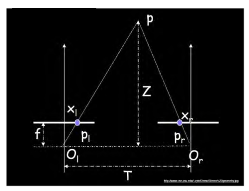
Assume parallel optical axes, known camera parameters (i.e., calibrated cameras). What is expression for Z?
|
||
|
||
Similar triangles $(p_l, P, p_r)$ and $(O_l, P, O_r)$:
|
||
|
||
$$
|
||
\frac{T-x_l+x_r}{Z-f}=\frac{T}{Z}
|
||
$$
|
||
|
||
$$
|
||
Z = \frac{f \cdot T}{x_l-x_r}
|
||
$$
|
||
|
||
### Camera Calibration
|
||
|
||
Use an scene with known geometry
|
||
|
||
- Correspond image points to 3d points
|
||
- Get least squares solution (or non-linear solution)
|
||
|
||
Solving unknown camera parameters:
|
||
|
||
$$
|
||
\begin{bmatrix}
|
||
su\\
|
||
sv\\
|
||
s
|
||
\end{bmatrix}
|
||
= \begin{bmatrix}
|
||
m_{11} & m_{12} & m_{13} & m_{14}\\
|
||
m_{21} & m_{22} & m_{23} & m_{24}\\
|
||
m_{31} & m_{32} & m_{33} & m_{34}
|
||
\end{bmatrix}
|
||
\begin{bmatrix}
|
||
X\\
|
||
Y\\
|
||
Z\\
|
||
1
|
||
\end{bmatrix}
|
||
$$
|
||
|
||
Method 1: Homogenous linear system. Solve for m's entries using least squares.
|
||
|
||
$$
|
||
\begin{bmatrix}
|
||
X_1 & Y_1 & Z_1 & 1 & 0 & 0 & 0 & 0 & -u_1X_1 & -u_1Y_1 & -u_1Z_1 & -u_1 \\
|
||
0 & 0 & 0 & 0 & X_1 & Y_1 & Z_1 & 1 & -v_1X_1 & -v_1Y_1 & -v_1Z_1 & -v_1 \\
|
||
\vdots & \vdots & \vdots & \vdots & \vdots & \vdots & \vdots & \vdots & \vdots & \vdots\\
|
||
X_n & Y_n & Z_n & 1 & 0 & 0 & 0 & 0 & -u_nX_n & -u_nY_n & -u_nZ_n & -u_n \\
|
||
0 & 0 & 0 & 0 & X_n & Y_n & Z_n & 1 & -v_nX_n & -v_nY_n & -v_nZ_n & -v_n
|
||
\end{bmatrix}
|
||
\begin{bmatrix} m_{11} \\ m_{12} \\ m_{13} \\ m_{14} \\ m_{21} \\ m_{22} \\ m_{23} \\ m_{24} \\ m_{31} \\ m_{32} \\ m_{33} \\ m_{34} \end{bmatrix} = 0
|
||
$$
|
||
|
||
Method 2: Non-homogenous linear system. Solve for m's entries using least squares.
|
||
|
||
**Advantages**
|
||
|
||
- Easy to formulate and solve
|
||
- Provides initialization for non-linear methods
|
||
|
||
**Disadvantages**
|
||
|
||
- Doesn't directly give you camera parameters
|
||
- Doesn't model radial distortion
|
||
- Can't impose constraints, such as known focal length
|
||
|
||
**Non-linear methods are preferred**
|
||
|
||
- Define error as difference between projected points and measured points
|
||
- Minimize error using Newton's method or other non-linear optimization
|
||
|
||
#### Triangulation
|
||
|
||
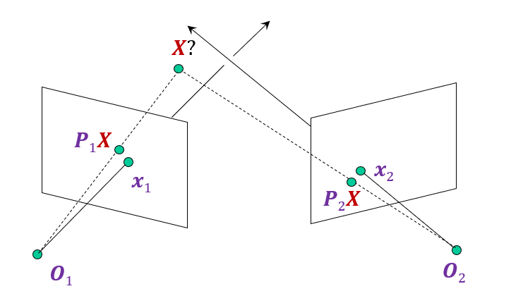
Given projections of a 3D point in two or more images (with known camera matrices), find the coordinates of the point
|
||
|
||
##### Approaches 1: Geometric approach
|
||
|
||
Find shortest segment connecting the two viewing rays and let $X$ be the midpoint of that segment
|
||
|
||
|
||
|
||
##### Approaches 2: Non-linear optimization
|
||
|
||
Minimize error between projected point and measured point
|
||
|
||
$$
|
||
||\operatorname{proj}(P_1 X) - x_1||_2^2 + ||\operatorname{proj}(P_2 X) - x_2||_2^2
|
||
$$
|
||
|
||
|
||
|
||
##### Approaches 3: Linear approach
|
||
|
||
$x_1\cong P_1X$ and $x_2\cong P_2X$
|
||
|
||
$x_1\times P_1X = 0$ and $x_2\times P_2X = 0$
|
||
|
||
$[x_{1_{\times}}]P_1X = 0$ and $[x_{2_{\times}}]P_2X = 0$
|
||
|
||
Rewrite as:
|
||
|
||
$$
|
||
a\times b=\begin{bmatrix}
|
||
0 & -a_3 & a_2\\
|
||
a_3 & 0 & -a_1\\
|
||
-a_2 & a_1 & 0
|
||
\end{bmatrix}
|
||
\begin{bmatrix}
|
||
b_1\\
|
||
b_2\\
|
||
b_3
|
||
\end{bmatrix}
|
||
=[a_{\times}]b
|
||
$$
|
||
|
||
Using **singular value decomposition**, we can solve for $X$
|
||
|
||
### Epipolar Geometry
|
||
|
||
What constraints must hold between two projections of the same 3D point?
|
||
|
||
Given a 2D point in one view, where can we find the corresponding point in the other view?
|
||
|
||
Given only 2D correspondences, how can we calibrate the two cameras, i.e., estimate their relative position and orientation and the intrinsic parameters?
|
||
|
||
Key ideas:
|
||
|
||
- We can answer all these questions without knowledge of the 3D scene geometry
|
||
- Important to think about projections of camera centers and visual rays into the other view
|
||
|
||
#### Epipolar Geometry Setup
|
||
|
||
|
||
|
||
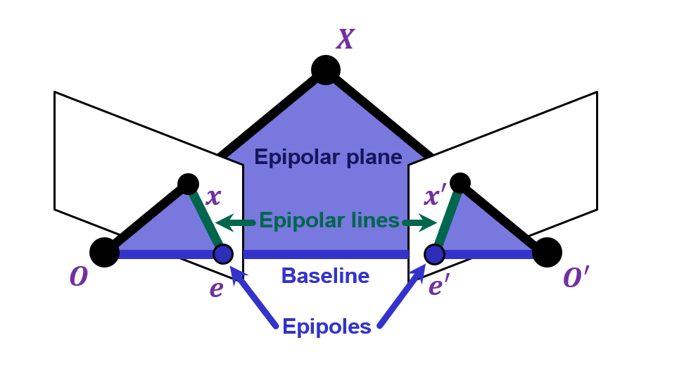
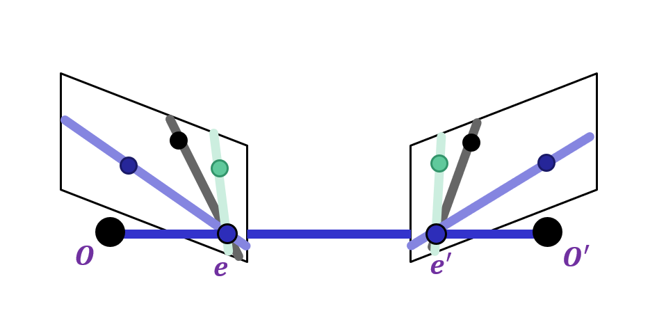
Suppose we have two cameras with centers $O,O'$
|
||
|
||
The baseline is the line connecting the origins
|
||
|
||
Epipoles $e,e'$ are where the baseline intersects the image planes, or projections of the other camera in each view
|
||
|
||
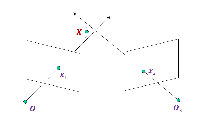
Consider a point $X$, which projects to $x$ and $x'$
|
||
|
||
The plane formed by $X,O,O'$ is called an epipolar plane
|
||
There is a family of planes passing through $O$ and $O'$
|
||
|
||
Epipolar lines are projections of the baseline into the image planes
|
||
|
||
**Epipolar lines** connect the epipoles to the projections of $X$
|
||
Equivalently, they are intersections of the epipolar plane with the image planes – thus, they come in matching pairs.
|
||
|
||
**Application**: This constraint can be used to find correspondences between points in two camera. by the epipolar line in one image, we can find the corresponding feature in the other image.
|
||
|
||
|
||
|
||
Epipoles are finite and may be visible in the image.
|
||
|
||
|
||
|
||
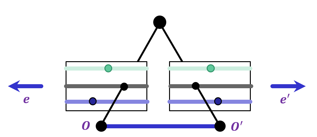
Epipoles are infinite, epipolar lines parallel.
|
||
|
||
|
||
|
||
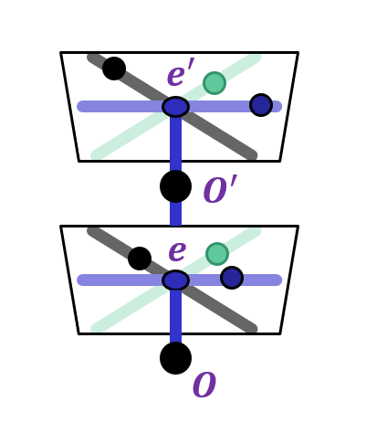
Epipole is "focus of expansion" and coincides with the principal point of the camera
|
||
|
||
Epipolar lines go out from principal point
|
||
|
||
Next class:
|
||
|
||
### The Essential and Fundamental Matrices
|
||
|
||
### Dense Stereo Matching
|
||
|
||
|