NoteNextra-origin/content/CSE559A/CSE559A_L6.md

CSE559A Lecture 6

Continue on Light, eye/camera, and color

BRDF (Bidirectional Reflectance Distribution Function)

\rho(\theta_i,\phi_i,\theta_o,\phi_o)

Diffuse Reflection

• Dull, matte surface like chalk or latex paint

• Most often used in computer vision

• Brightness does depend on direction of illumination

Diffuse reflection governed by Lambert's law: I_d = k_d N\cdot L I_i

• N: surface normal
• L: light direction
• I_i: incident light intensity
• k_d: albedo

\rho(\theta_i,\phi_i,\theta_o,\phi_o)=k_d \cos\theta_i

Photometric Stereo

Suppose there are three light sources, L_1, L_2, L_3, and we have the following measurements:

I_1 = k_d N\cdot L_1

I_2 = k_d N\cdot L_2

I_3 = k_d N\cdot L_3

We can solve for N by taking the dot product of N and each light direction and then solving the system of equations.

Will not do this in the lecture.

Specular Reflection

• Mirror-like surface

I_e=\begin{cases}
I_i & \text{if } V=R \\
0 & \text{if } V\neq R
\end{cases}

• V: view direction
• R: reflection direction
• \theta_i: angle between the incident light and the surface normal

Near-perfect mirror have a high light around R.

common model:

I_e=k_s (V\cdot R)^{n_s}I_i

• k_s: specular reflection coefficient
• n_s: shininess (imperfection of the surface)
• I_i: incident light intensity

Phong illumination model

• Phong approximation of surface reflectance
  • Assume reflectance is modeled by three compoents
    • Diffuse reflection
    • Specular reflection
    • Ambient reflection

I_e=k_a I_a + I_i \left[k_d (N\cdot L) + k_s (V\cdot R)^{n_s}\right]

• k_a: ambient reflection coefficient
• I_a: ambient light intensity
• k_d: diffuse reflection coefficient
• k_s: specular reflection coefficient
• n_s: shininess
• I_i: incident light intensity

Many other models.

Measuring BRDF

Use Gonioreflectometer.

• Device for measuring the reflectance of a surface as a function of the incident and reflected angles.
• Can be used to measure the BRDF of a surface.

BRDF dataset:

• MERL dataset
• CURET dataset

Camera/Eye

DSLR Camera

• Pinhole camera model
• Lens
• Aperture (the pinhole)
• Sensor
• ...

Digital Camera block diagram

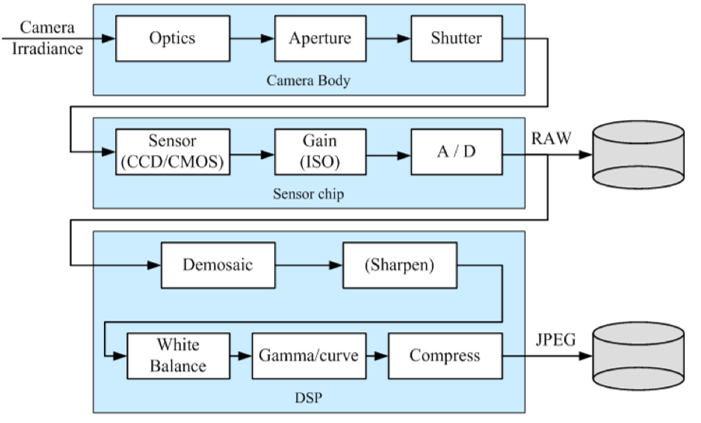
Scanning protocols:

• Global shutter: all pixels are exposed at the same time
• Interlaced: odd and even lines are exposed at different times
• Rolling shutter: each line is exposed as it is read out

Eye

• Pupil
• Iris
• Retina
• Rods and cones
• ...

Eye Movements

• Saccade
  • Can be consciously controlled. Related to perceptual attention.
  • 200ms to initiation, 20 to 200ms to carry out. Large amplitude.
• Smooth pursuit
  • Tracking an object
  • Difficult w/o an object to track!
• Microsaccade and Ocular microtremor (OMT)
  • Involuntary. Smaller amplitude. Especially evident during prolonged fixation.

Contrast Sensitivity

• Uniform contrast image content, with increasing frequency
• Why not uniform across the top?
• Low frequencies: harder to see because of slower intensity changes
• Higher frequencies: harder to see because of ability of our visual system to resolve fine features

Color Perception

Visible light spectrum: 380 to 780 nm

• 400 to 500 nm: blue
• 500 to 600 nm: green
• 600 to 700 nm: red

HSV model

We use Gaussian functions to model the sensitivity of the human eye to different wavelengths.

• Hue: color (the wavelength of the highest peak of the sensitivity curve)
• Saturation: color purity (the variance of the sensitivity curve)
• Value: color brightness (the highest peak of the sensitivity curve)

Color Sensing in Camera (RGB)

• 3-chip vs. 1-chip: quality vs. cost

Bayer filter:

• Why more green?
  • Human eye is more sensitive to green light.

Color spaces

Images in python:

As matrix.

import matplotlib.pyplot as plt

from mpl_toolkits.mplot3d import Axes3D
from skimage import io

def plot_rgb_3d(image_path):
    image = io.imread(image_path)
    r, g, b = image[:,:,0], image[:,:,1], image[:,:,2]
    fig = plt.figure()
    ax = fig.add_subplot(111, projection='3d')
    ax.scatter(r.flatten(), g.flatten(), b.flatten(), c=image.reshape(-1, 3)/255.0, marker='.')
    ax.set_xlabel('Red')
    ax.set_ylabel('Green')
    ax.set_zlabel('Blue')
    plt.show()

plot_rgb_3d('image.jpg')

Other color spaces:

• YCbCr (fast to compute, usually used in TV)
• HSV
• L*a*b* (CIELAB, perceptually uniform color space)

Most information is in the intensity channel.